Chapter 23: Building a CNN from Scratch

Chapter 23: Building a CNN from Scratch#

In Part V we built a fully-connected neural network from the ground up. Every input neuron was connected to every hidden neuron – a sensible choice for small, unstructured inputs. But images have spatial structure: nearby pixels are related, and the same edge or texture can appear anywhere in the field of view. A convolutional neural network (CNN) exploits this structure by replacing the dense matrix multiply with a local, sliding-window operation called convolution.

In this chapter we assemble all the building blocks of a small CNN:

Conv2D – the convolutional layer (defined in Chapter 22),
ReLU – the nonlinearity inserted after each convolution,
MaxPool2D – spatial downsampling that preserves the strongest activations,
Flatten and Dense – the bridge from spatial feature maps to class scores.

We then combine them into a complete TinyCNN class and generate a synthetic dataset of oriented line patterns to test it on.

Prerequisites

This chapter assumes familiarity with the Conv2D layer introduced in Chapter 22. All code is pure NumPy – no deep learning frameworks are used.

We begin by defining the Conv2D layer. In this chapter we implement only the forward pass; the backward pass (needed for training) will be derived and implemented in Chapter 24.

Definition (2D Convolution Layer)

A Conv2D layer with \(C_{\text{out}}\) filters of size \(k \times k\) applied to an input with \(C_{\text{in}}\) channels computes

\[y_{f,i,j} = b_f + \sum_{c=1}^{C_{\text{in}}} \sum_{p=0}^{k-1} \sum_{q=0}^{k-1} K_{f,c,p,q} \cdot x_{c,\, i+p,\, j+q}\]

for each filter \(f = 1, \ldots, C_{\text{out}}\) and each valid spatial position \((i, j)\). The output spatial dimensions are \(H_{\text{out}} = H - k + 1\) and \(W_{\text{out}} = W - k + 1\) (no padding, stride 1).

class Conv2D:
    """2D convolutional layer (forward pass only).
    
    Parameters
    ----------
    in_channels : int
        Number of input channels.
    out_channels : int
        Number of filters (output channels).
    kernel_size : int
        Spatial size of each filter (kernel_size x kernel_size).
    seed : int
        Random seed for reproducibility.
    """
    def __init__(self, in_channels, out_channels, kernel_size, seed=42):
        rng = np.random.default_rng(seed)
        fan_in = in_channels * kernel_size * kernel_size
        scale = np.sqrt(2.0 / fan_in)          # He initialization
        self.in_channels = in_channels
        self.out_channels = out_channels
        self.kernel_size = kernel_size
        self.weights = rng.normal(0.0, scale,
                                  size=(out_channels, in_channels,
                                        kernel_size, kernel_size))
        self.bias = np.zeros(out_channels)
        self.last_input = None                  # cached for backward (ch24)

    def forward(self, x):
        """Slide each filter across the input and accumulate dot products.
        
        Parameters
        ----------
        x : ndarray, shape (batch, in_channels, height, width)
        
        Returns
        -------
        output : ndarray, shape (batch, out_channels, out_h, out_w)
        """
        self.last_input = x
        batch_size, _, height, width = x.shape
        out_h = height - self.kernel_size + 1
        out_w = width - self.kernel_size + 1
        output = np.zeros((batch_size, self.out_channels, out_h, out_w))
        for row in range(out_h):
            for col in range(out_w):
                patch = x[:, :,
                          row:row + self.kernel_size,
                          col:col + self.kernel_size]
                # tensordot over (in_channels, kH, kW) axes
                output[:, :, row, col] = (
                    np.tensordot(patch, self.weights,
                                 axes=([1, 2, 3], [1, 2, 3]))
                    + self.bias
                )
        return output

    @property
    def parameter_count(self):
        return int(self.weights.size + self.bias.size)


print("Conv2D class defined (forward only).")
print("Attributes: weights, bias, last_input")
print("Methods: forward, parameter_count")

Conv2D class defined (forward only).
Attributes: weights, bias, last_input
Methods: forward, parameter_count

23.1 ReLU After Convolution#

A convolution is a linear operation: it computes weighted sums over local patches. Stacking two linear operations without a nonlinearity in between collapses to a single linear operation – exactly the lesson of Chapter 8 (the XOR problem). To build depth that matters, we insert a rectified linear unit (ReLU) after every convolution:

\[\text{ReLU}(z) = \max(0, z).\]

Why ReLU?

ReLU is the default activation in modern CNNs for three reasons:

Sparse activation – roughly half the units output zero, yielding efficient representations.
No vanishing gradient – the gradient is either 0 or 1, so deep networks train easily.
Computational simplicity – a single comparison, much cheaper than sigmoid or tanh.

class ReLU:
    """Element-wise Rectified Linear Unit."""
    def __init__(self):
        self.last_input = None

    def forward(self, x):
        self.last_input = x
        return np.maximum(0.0, x)

    def backward(self, d_output):
        return d_output * (self.last_input > 0.0)


print("ReLU class defined.")
print("forward:  max(0, x)")
print("backward: pass gradient where x > 0, zero elsewhere")

ReLU class defined.
forward:  max(0, x)
backward: pass gradient where x > 0, zero elsewhere

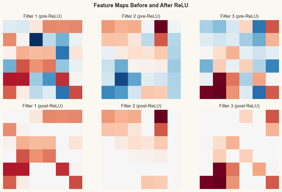
The figure below shows what happens to a feature map before and after ReLU. All negative activations are set to zero, producing a sparser representation.

../_images/d22db53d3a2bd268ebedc1de48b96ba5a11e7e5ebd59b82c1e0108017d8a751b.png

23.2 Max Pooling#

After the convolution + ReLU pair has extracted local features, we want to downsample the feature maps. This serves two purposes:

Reduce computation – fewer spatial positions means fewer operations in later layers.
Translation invariance – small shifts in the input do not change the pooled output.

Definition (Max Pooling)

Max pooling with pool size \(p\) partitions each channel of the feature map into non-overlapping \(p \times p\) windows and replaces each window with its maximum value:

\[y_{c,i,j} = \max_{0 \le r,s < p}\; x_{c,\, ip+r,\, jp+s}\]

The output spatial dimensions are \(H_{\text{out}} = \lfloor H/p \rfloor\) and \(W_{\text{out}} = \lfloor W/p \rfloor\).

Tip

Max pooling retains the strongest activation in each window, discarding precise spatial location. This is exactly the trade-off we want: “Is there an edge somewhere in this region?” rather than “Is there an edge at pixel \((3, 7)\)?”

class MaxPool2D:
    """Max pooling with non-overlapping windows.
    
    Parameters
    ----------
    pool_size : int
        Side length of each pooling window.
    """
    def __init__(self, pool_size=2):
        self.pool_size = pool_size
        self.last_input = None
        self.last_mask = None      # records winner positions for backward

    def forward(self, x):
        self.last_input = x
        batch_size, channels, height, width = x.shape
        out_h = height // self.pool_size
        out_w = width // self.pool_size
        output = np.zeros((batch_size, channels, out_h, out_w))
        mask = np.zeros_like(x)
        for row in range(out_h):
            for col in range(out_w):
                rs = row * self.pool_size
                cs = col * self.pool_size
                window = x[:, :, rs:rs + self.pool_size,
                                  cs:cs + self.pool_size]
                output[:, :, row, col] = window.max(axis=(2, 3))
                flat_idx = window.reshape(
                    batch_size, channels, -1).argmax(axis=2)
                for b in range(batch_size):
                    for c in range(channels):
                        winner = flat_idx[b, c]
                        wr = winner // self.pool_size
                        wc = winner % self.pool_size
                        mask[b, c, rs + wr, cs + wc] = 1.0
        self.last_mask = mask
        return output

    def backward(self, d_output):
        d_input = np.zeros_like(self.last_input)
        out_h, out_w = d_output.shape[2], d_output.shape[3]
        for row in range(out_h):
            for col in range(out_w):
                rs = row * self.pool_size
                cs = col * self.pool_size
                mask_w = self.last_mask[
                    :, :, rs:rs + self.pool_size,
                          cs:cs + self.pool_size]
                d_input[:, :, rs:rs + self.pool_size,
                              cs:cs + self.pool_size] += (
                    mask_w * d_output[:, :, row, col][:, :, None, None]
                )
        return d_input


print("MaxPool2D class defined.")
print("forward:  take the max in each pool_size x pool_size window")
print("backward: route gradient only to the max position")

MaxPool2D class defined.
forward:  take the max in each pool_size x pool_size window
backward: route gradient only to the max position

../_images/f43da0a75014204276feb5bf8b70056dd8bff0b8c2db1dbddacfac20c3fa69a6.png

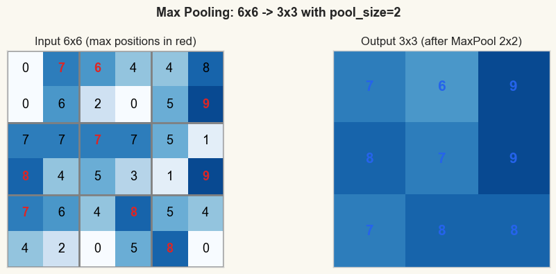
Each 2x2 block is replaced by its maximum value.
The spatial resolution is halved in each dimension.

23.3 Flatten and Dense#

After convolution, ReLU, and pooling, we have a 3-D tensor of shape (batch, channels, height, width). To produce class scores we need a fully-connected (dense) layer, which expects a 1-D vector per sample. The Flatten layer reshapes the spatial feature maps into a flat vector:

\[(B, C, H, W) \longrightarrow (B, C \cdot H \cdot W).\]

The Dense layer then computes the familiar linear transformation:

\[\mathbf{y} = \bx \bW + \bb\]

where \(\bW \in \mathbb{R}^{D_{\text{in}} \times D_{\text{out}}}\) and \(\bb \in \mathbb{R}^{D_{\text{out}}}\).

class Flatten:
    """Reshape a 4-D tensor to 2-D (batch, features)."""
    def __init__(self):
        self.last_shape = None

    def forward(self, x):
        self.last_shape = x.shape
        return x.reshape(x.shape[0], -1)

    def backward(self, d_output):
        return d_output.reshape(self.last_shape)


class Dense:
    """Fully-connected layer (forward pass only in this chapter).
    
    Parameters
    ----------
    in_features : int
        Dimensionality of each input vector.
    out_features : int
        Number of output units.
    seed : int
        Random seed for reproducibility.
    """
    def __init__(self, in_features, out_features, seed=42):
        rng = np.random.default_rng(seed)
        scale = np.sqrt(2.0 / in_features)  # He initialization
        self.weights = rng.normal(0.0, scale,
                                  size=(in_features, out_features))
        self.bias = np.zeros(out_features)
        self.last_input = None

    def forward(self, x):
        self.last_input = x
        return x @ self.weights + self.bias

    @property
    def parameter_count(self):
        return int(self.weights.size + self.bias.size)


print("Flatten and Dense classes defined (forward only).")
print("Flatten: (B, C, H, W) -> (B, C*H*W)")
print("Dense:   y = x @ W + b")

Flatten and Dense classes defined (forward only).
Flatten: (B, C, H, W) -> (B, C*H*W)
Dense:   y = x @ W + b

We also need the softmax function and the cross-entropy loss for multi-class classification. These are identical to what we would use in a fully-connected network.

def softmax(logits):
    """Numerically stable softmax.
    
    Parameters
    ----------
    logits : ndarray, shape (batch, num_classes)
    
    Returns
    -------
    probabilities : ndarray, same shape as logits
    """
    shifted = logits - logits.max(axis=1, keepdims=True)
    exp_values = np.exp(shifted)
    return exp_values / exp_values.sum(axis=1, keepdims=True)


def softmax_cross_entropy(logits, targets):
    """Combined softmax + cross-entropy loss.
    
    Parameters
    ----------
    logits : ndarray, shape (batch, num_classes)
    targets : ndarray of int, shape (batch,)
    
    Returns
    -------
    loss : float
    probabilities : ndarray, shape (batch, num_classes)
    d_logits : ndarray, shape (batch, num_classes)
    """
    probabilities = softmax(logits)
    batch_idx = np.arange(targets.shape[0])
    clipped = np.clip(probabilities[batch_idx, targets], 1e-12, 1.0)
    loss = -np.log(clipped).mean()
    d_logits = probabilities.copy()
    d_logits[batch_idx, targets] -= 1.0
    d_logits /= targets.shape[0]
    return loss, probabilities, d_logits


print("softmax and softmax_cross_entropy defined.")

softmax and softmax_cross_entropy defined.

23.4 The TinyCNN Class#

We now assemble the pieces into a complete network. Our architecture is deliberately small so that it trains in seconds on the CPU:

\[\text{Input}(1, 8, 8) \;\xrightarrow{\text{Conv2D}(1{\to}3,\; 3{\times}3)}\; (3, 6, 6) \;\xrightarrow{\text{ReLU}}\; (3, 6, 6) \;\xrightarrow{\text{MaxPool}(2)}\; (3, 3, 3) \;\xrightarrow{\text{Flatten}}\; (27) \;\xrightarrow{\text{Dense}(27{\to}3)}\; (3)\]

Architecture Summary

TinyCNN has five layers:

Conv2D(1, 3, 3) – 3 filters of size \(3 \times 3\) on 1 input channel
ReLU – element-wise nonlinearity
MaxPool2D(2) – \(2 \times 2\) max pooling
Flatten – reshape \((3, 3, 3) \to (27)\)
Dense(27, 3) – fully-connected layer producing 3 class scores

class TinyCNN:
    """A minimal convolutional neural network for 8x8 grayscale images.
    
    Architecture:
        Conv2D(1->3, 3x3) -> ReLU -> MaxPool(2x2) -> Flatten -> Dense(27->3)
    """
    def __init__(self, seed=42):
        self.conv = Conv2D(in_channels=1, out_channels=3,
                           kernel_size=3, seed=seed)
        self.relu = ReLU()
        self.pool = MaxPool2D(pool_size=2)
        self.flatten = Flatten()
        self.dense = Dense(in_features=27, out_features=3,
                           seed=seed + 1)
        self.layers = [self.conv, self.relu, self.pool,
                       self.flatten, self.dense]

    def forward(self, x):
        """Forward pass through all layers."""
        for layer in self.layers:
            x = layer.forward(x)
        return x  # logits, shape (batch, 3)

    def predict(self, x):
        """Return predicted class indices."""
        logits = self.forward(x)
        return np.argmax(logits, axis=1)

    def evaluate(self, x, y):
        """Compute accuracy on a dataset."""
        preds = self.predict(x)
        return np.mean(preds == y)


print("TinyCNN class defined.")
print("Architecture: Conv2D(1->3, 3x3) -> ReLU -> MaxPool(2) -> Flatten -> Dense(27->3)")
print("Methods: forward, predict, evaluate")

TinyCNN class defined.
Architecture: Conv2D(1->3, 3x3) -> ReLU -> MaxPool(2) -> Flatten -> Dense(27->3)
Methods: forward, predict, evaluate

23.5 Layer Summary#

Let us verify the shapes and count the parameters at each stage.

Layer        Output Shape           Parameters
==============================================
Input        (1, 1, 8, 8)                    -
Conv2D       (1, 3, 6, 6)                   30
ReLU         (1, 3, 6, 6)                    -
MaxPool2D    (1, 3, 3, 3)                    -
Flatten      (1, 27)                         -
Dense        (1, 3)                         84
==============================================
TOTAL                                      114

Conv2D:  3 filters x (1 x 3 x 3) + 3 biases = 30
Dense:   27 x 3 weights + 3 biases = 84
Total trainable parameters: 114

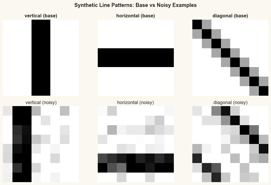
23.6 The Synthetic Dataset#

To test our TinyCNN we create a simple dataset of \(8 \times 8\) grayscale images containing three classes of oriented line patterns:

vertical – a vertical bar through the center,
horizontal – a horizontal bar through the center,
diagonal – a diagonal line from top-left to bottom-right.

Each training example is generated by taking the base pattern, applying random vertical/horizontal shifts, and adding Gaussian noise. This mimics the kind of translation variability that makes CNNs superior to fully-connected networks.

Why Synthetic Data?

Using synthetic data lets us control exactly what the network must learn. We know the ground truth – three oriented patterns – so we can later inspect whether the learned filters match these orientations.

CLASS_NAMES = ("vertical", "horizontal", "diagonal")


def _pattern_for_class(class_name, size):
    """Generate the base pattern for a given class."""
    pattern = np.zeros((size, size))
    center = size // 2
    if class_name == "vertical":
        pattern[:, center - 1:center + 1] = 1.0
    elif class_name == "horizontal":
        pattern[center - 1:center + 1, :] = 1.0
    elif class_name == "diagonal":
        np.fill_diagonal(pattern, 1.0)
        pattern += 0.35 * np.eye(size, k=1)
        pattern += 0.35 * np.eye(size, k=-1)
    return np.clip(pattern, 0.0, 1.0)


def make_dataset_bundle(train_per_class=60, val_per_class=30,
                         size=8, seed=7, class_names=CLASS_NAMES):
    """Generate shifted, noisy variants of base patterns.
    
    Returns
    -------
    x_train : ndarray, shape (N_train, 1, size, size)
    y_train : ndarray of int, shape (N_train,)
    x_val : ndarray, shape (N_val, 1, size, size)
    y_val : ndarray of int, shape (N_val,)
    class_names : tuple of str
    """
    rng = np.random.default_rng(seed)
    all_x, all_y = [], []
    total_per_class = train_per_class + val_per_class

    for cls_idx, cls_name in enumerate(class_names):
        base = _pattern_for_class(cls_name, size)
        for _ in range(total_per_class):
            # Random shift
            shift_r = rng.integers(-2, 3)
            shift_c = rng.integers(-2, 3)
            shifted = np.roll(np.roll(base, shift_r, axis=0),
                              shift_c, axis=1)
            # Add noise
            noisy = shifted + rng.normal(0, 0.15, size=(size, size))
            noisy = np.clip(noisy, 0.0, 1.0)
            all_x.append(noisy)
            all_y.append(cls_idx)

    all_x = np.array(all_x)[:, None, :, :]   # (N, 1, 8, 8)
    all_y = np.array(all_y, dtype=int)

    # Shuffle and split
    perm = rng.permutation(len(all_y))
    all_x, all_y = all_x[perm], all_y[perm]

    n_train = train_per_class * len(class_names)
    x_train, y_train = all_x[:n_train], all_y[:n_train]
    x_val, y_val = all_x[n_train:], all_y[n_train:]

    return x_train, y_train, x_val, y_val, class_names


# Generate the dataset
x_train, y_train, x_val, y_val, class_names = make_dataset_bundle()

print(f"Training set:   {x_train.shape[0]} images, shape {x_train.shape[1:]}")
print(f"Validation set: {x_val.shape[0]} images, shape {x_val.shape[1:]}")
print(f"Classes: {class_names}")
for i, name in enumerate(class_names):
    n_tr = (y_train == i).sum()
    n_va = (y_val == i).sum()
    print(f"  {name}: {n_tr} train, {n_va} val")

Training set:   180 images, shape (1, 8, 8)
Validation set: 90 images, shape (1, 8, 8)
Classes: ('vertical', 'horizontal', 'diagonal')
  vertical: 67 train, 23 val
  horizontal: 54 train, 36 val
  diagonal: 59 train, 31 val

../_images/a26d0eb48591f271edb6e4d7dee7ce7d67c1e79f59d426e2a0821435dc0e4e14.png

Let us verify that the untrained TinyCNN produces essentially random predictions:

Untrained TinyCNN accuracy:
  Train: 38.3%  (chance = 33.3%)
  Val:   40.0%

The network needs training! That is the subject of Chapter 24.

Exercises#

Exercise 23.1. Compute the output shape of a Conv2D layer with in_channels=3, out_channels=8, kernel_size=5 applied to an input of shape (16, 3, 32, 32). How many parameters does this layer have?

Exercise 23.2. What happens if we remove the ReLU between convolution and pooling? Explain why the network’s representational power would be affected, connecting your answer to the XOR impossibility result of Chapter 8.

Exercise 23.3. Average pooling replaces each window with its mean instead of its maximum. Implement an AvgPool2D class with forward and backward methods. What is the backward pass of average pooling?

Exercise 23.4. Add a fourth class "dot" (a 2x2 square in the center) to the dataset. What changes are needed in the TinyCNN architecture? Modify the code and verify that the shapes are consistent.

Exercise 23.5. Our TinyCNN has about 114 parameters. A fully-connected network mapping 64 inputs to 3 outputs through a hidden layer of 27 neurons would have \(64 \times 27 + 27 + 27 \times 3 + 3 = 1839\) parameters. Explain the source of this large difference and discuss the concept of parameter sharing in CNNs.