Chapter 15: Gradient Descent Foundations#
Having established the limitations of Hebbian learning (Part 4), we now turn to supervised learning, where the goal is to minimize a loss function that measures the discrepancy between the network’s output and a target. This chapter develops the mathematical foundations of gradient descent, the optimization algorithm that underlies all of modern deep learning.
15.1 Optimization as a Framework#
The Supervised Learning Setup#
Given:
A training set \(\{(\mathbf{x}^{(1)}, \mathbf{y}^{(1)}), \ldots, (\mathbf{x}^{(N)}, \mathbf{y}^{(N)})\}\)
A parameterized model \(f(\mathbf{x}; \mathbf{w})\) with parameters \(\mathbf{w}\)
A loss function \(L(\hat{\mathbf{y}}, \mathbf{y})\) measuring prediction quality
The empirical risk minimization problem is:
This frames learning as an optimization problem. The model “learns” by finding parameters that minimize the average loss over the training data.
15.2 The Gradient#
Definition#
For a differentiable function \(\mathcal{L}: \mathbb{R}^n \to \mathbb{R}\), the gradient at point \(\mathbf{w}\) is the vector of partial derivatives:
Key Property#
The gradient points in the direction of steepest ascent of \(\mathcal{L}\).
Proof: Consider the directional derivative of \(\mathcal{L}\) in direction \(\mathbf{v}\) (\(\|\mathbf{v}\| = 1\)):
where \(\theta\) is the angle between \(\nabla \mathcal{L}\) and \(\mathbf{v}\). This is maximized when \(\theta = 0\), i.e., \(\mathbf{v} = \nabla \mathcal{L} / \|\nabla \mathcal{L}\|\). \(\blacksquare\)
Corollary: The direction of steepest descent is \(-\nabla \mathcal{L}\).
15.3 The Gradient Descent Update Rule#
To minimize \(\mathcal{L}(\mathbf{w})\), we iteratively move in the direction of steepest descent:
Algorithm (Gradient Descent)
Input: Initial parameters \(\mathbf{w}_0\), learning rate \(\eta > 0\), number of iterations \(T\)
For \(t = 0, 1, \ldots, T-1\):
Output: Final parameters \(\mathbf{w}_T\)
The learning rate \(\eta > 0\) controls the step size. At each iteration, compute the full gradient over all training examples and take a step in the negative gradient direction.
Intuition#
Imagine standing on a mountainside in fog. You can feel the slope beneath your feet (the gradient) but cannot see the valley. Gradient descent says: take a step downhill proportional to the steepness of the slope.
Show code cell source
import numpy as np
import matplotlib.pyplot as plt
from matplotlib import cm

# Visualize gradient descent on two 2D functions

fig, axes = plt.subplots(1, 2, figsize=(16, 7))

# ---- Function 1: Quadratic Bowl ----
# L(w1, w2) = w1^2 + 5*w2^2
def quadratic(w):
    return w[0]**2 + 5*w[1]**2

def grad_quadratic(w):
    return np.array([2*w[0], 10*w[1]])

# Grid for contour
w1 = np.linspace(-5, 5, 200)
w2 = np.linspace(-3, 3, 200)
W1, W2 = np.meshgrid(w1, w2)
Z = W1**2 + 5*W2**2

axes[0].contour(W1, W2, Z, levels=20, cmap='viridis', alpha=0.6)
axes[0].set_xlabel('$w_1$', fontsize=12)
axes[0].set_ylabel('$w_2$', fontsize=12)
axes[0].set_title('Quadratic: $L = w_1^2 + 5w_2^2$', fontsize=13)

# Gradient descent
eta = 0.08
w = np.array([4.0, 2.5])
trajectory = [w.copy()]
for _ in range(30):
    g = grad_quadratic(w)
    w = w - eta * g
    trajectory.append(w.copy())
trajectory = np.array(trajectory)

axes[0].plot(trajectory[:, 0], trajectory[:, 1], 'ro-', markersize=4, linewidth=1.5, label=f'GD ($\\eta={eta}$)')
axes[0].plot(0, 0, 'g*', markersize=15, label='Minimum')
axes[0].legend(fontsize=10)
axes[0].grid(True, alpha=0.2)

# ---- Function 2: Rosenbrock ----
# L(w1, w2) = (1 - w1)^2 + 100*(w2 - w1^2)^2
def rosenbrock(w):
    return (1 - w[0])**2 + 100*(w[1] - w[0]**2)**2

def grad_rosenbrock(w):
    dw1 = -2*(1 - w[0]) + 200*(w[1] - w[0]**2)*(-2*w[0])
    dw2 = 200*(w[1] - w[0]**2)
    return np.array([dw1, dw2])

w1r = np.linspace(-2, 2, 300)
w2r = np.linspace(-1, 3, 300)
W1R, W2R = np.meshgrid(w1r, w2r)
ZR = (1 - W1R)**2 + 100*(W2R - W1R**2)**2

axes[1].contour(W1R, W2R, np.log1p(ZR), levels=30, cmap='viridis', alpha=0.6)
axes[1].set_xlabel('$w_1$', fontsize=12)
axes[1].set_ylabel('$w_2$', fontsize=12)
axes[1].set_title('Rosenbrock: $L = (1-w_1)^2 + 100(w_2-w_1^2)^2$', fontsize=13)

# Gradient descent on Rosenbrock
eta_r = 0.001
w = np.array([-1.5, 2.0])
trajectory_r = [w.copy()]
for _ in range(5000):
    g = grad_rosenbrock(w)
    # Clip gradient for stability
    g = np.clip(g, -10, 10)
    w = w - eta_r * g
    trajectory_r.append(w.copy())
trajectory_r = np.array(trajectory_r)

# Plot every 50th point for clarity
axes[1].plot(trajectory_r[::50, 0], trajectory_r[::50, 1], 'ro-', markersize=3, linewidth=1, label=f'GD ($\\eta={eta_r}$)')
axes[1].plot(1, 1, 'g*', markersize=15, label='Minimum (1,1)')
axes[1].legend(fontsize=10)
axes[1].grid(True, alpha=0.2)

plt.tight_layout()
plt.savefig('gradient_descent_2d.png', dpi=150, bbox_inches='tight')
plt.show()

print(f"Quadratic: final point = ({trajectory[-1, 0]:.4f}, {trajectory[-1, 1]:.4f}), loss = {quadratic(trajectory[-1]):.6f}")
print(f"Rosenbrock: final point = ({trajectory_r[-1, 0]:.4f}, {trajectory_r[-1, 1]:.4f}), loss = {rosenbrock(trajectory_r[-1]):.6f}")

Quadratic: final point = (0.0214, 0.0000), loss = 0.000458
Rosenbrock: final point = (0.9181, 0.8425), loss = 0.006724
15.4 Convex vs Non-Convex Optimization#
Convex Functions#
A function \(\mathcal{L}\) is convex if for all \(\mathbf{w}_1, \mathbf{w}_2\) and \(\lambda \in [0,1]\):
For convex functions: every local minimum is a global minimum, and gradient descent converges to the global minimum (with appropriate learning rate).
Examples: Linear regression with MSE loss is convex.
Non-Convex Functions#
Neural network loss landscapes are almost always non-convex:
Multiple local minima
Saddle points (critical points where some directions curve up and others down)
Flat regions (plateaus)
Gradient descent on non-convex functions:
May converge to local minima (not global)
May get stuck at saddle points
Solution depends on initialization
Remarkable empirical finding: Despite non-convexity, gradient descent works well on neural networks in practice. Current understanding suggests that most local minima in high-dimensional loss landscapes are nearly as good as the global minimum (Choromanska et al., 2015).
Danger
❗ Local minima and saddle points – gradient descent finds LOCAL not GLOBAL minima. For non-convex loss surfaces (which neural networks have), there is NO guarantee of finding the optimal solution. The algorithm’s final point depends entirely on initialization and the learning rate.
Tip
The loss landscape of neural networks is surprisingly benign – most local minima are nearly as good as the global minimum. Recent research (Choromanska et al., 2015; Li et al., 2018) suggests that in high dimensions, saddle points are more problematic than local minima, and most critical points with high loss are saddle points, not local minima.
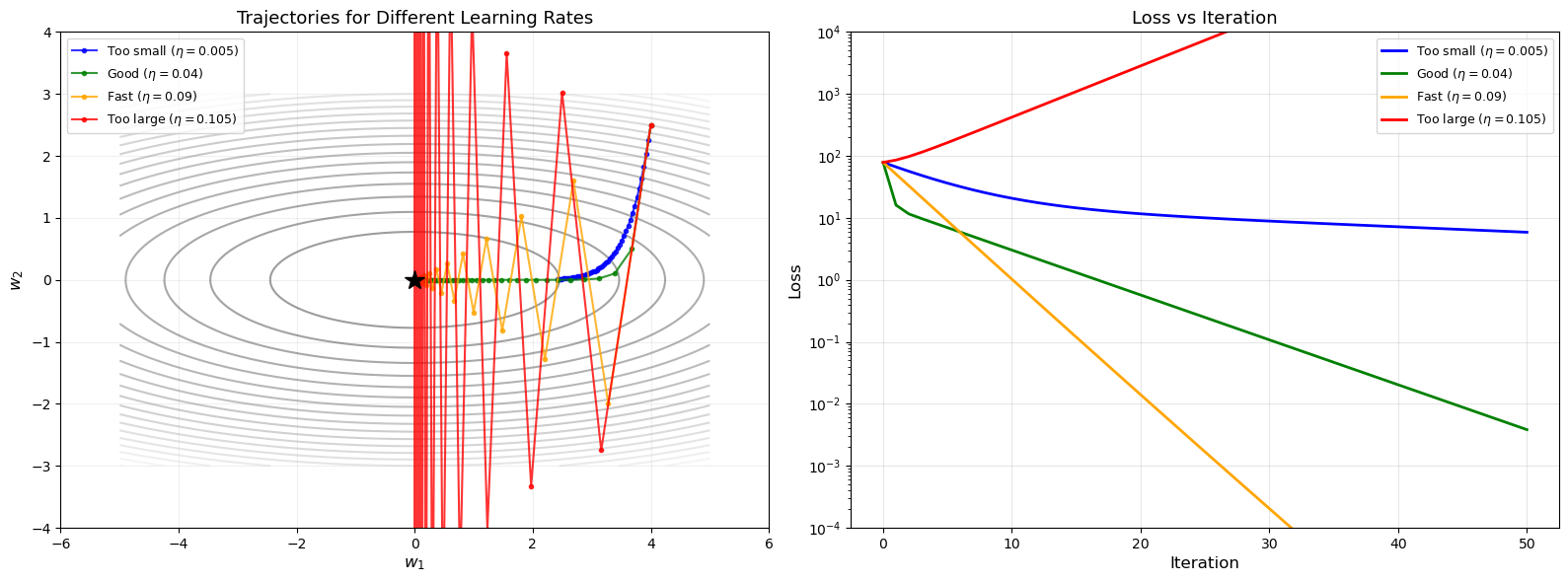
15.5 The Learning Rate#
The learning rate \(\eta\) is the most critical hyperparameter in gradient descent.
Too Large#
If \(\eta\) is too large, the updates overshoot the minimum, potentially causing divergence: the loss oscillates or increases without bound.
Too Small#
If \(\eta\) is too small, convergence is extremely slow. The algorithm may take an impractical number of iterations to reach an acceptable solution.
The Goldilocks Zone#
For a quadratic loss \(\mathcal{L}(\mathbf{w}) = \frac{1}{2}\mathbf{w}^\top \mathbf{H} \mathbf{w}\) with Hessian \(\mathbf{H}\) having eigenvalues \(\lambda_{\min}\) and \(\lambda_{\max}\):
Convergence requires \(\eta < 2/\lambda_{\max}\)
Optimal learning rate: \(\eta^* = 2/(\lambda_{\min} + \lambda_{\max})\)
Convergence rate depends on the condition number \(\kappa = \lambda_{\max}/\lambda_{\min}\)
Warning
Learning rate sensitivity – Too large: the optimization diverges (loss explodes or oscillates wildly). Too small: convergence is extremely slow, potentially requiring millions of iterations. There is no universal “best” learning rate; it depends on the loss landscape and must be tuned carefully.
Show code cell source
# Effect of learning rate: animate trajectory for different eta values

import numpy as np
import matplotlib.pyplot as plt

def quadratic_loss(w):
    return w[0]**2 + 10*w[1]**2

def quadratic_grad(w):
    return np.array([2*w[0], 20*w[1]])

etas = [0.005, 0.04, 0.09, 0.105]
labels = ['Too small ($\\eta=0.005$)', 'Good ($\\eta=0.04$)',
          'Fast ($\\eta=0.09$)', 'Too large ($\\eta=0.105$)']
colors = ['blue', 'green', 'orange', 'red']

fig, axes = plt.subplots(1, 2, figsize=(16, 6))

# Contour plot with trajectories
w1 = np.linspace(-5, 5, 200)
w2 = np.linspace(-3, 3, 200)
W1, W2 = np.meshgrid(w1, w2)
Z = W1**2 + 10*W2**2

axes[0].contour(W1, W2, Z, levels=20, cmap='gray', alpha=0.4)

all_losses = []
for eta, label, color in zip(etas, labels, colors):
    w = np.array([4.0, 2.5])
    traj = [w.copy()]
    losses = [quadratic_loss(w)]
    for _ in range(50):
        g = quadratic_grad(w)
        w = w - eta * g
        traj.append(w.copy())
        losses.append(quadratic_loss(w))
        if np.linalg.norm(w) > 100:
            break
    traj = np.array(traj)
    axes[0].plot(traj[:, 0], traj[:, 1], 'o-', color=color, markersize=3,
                 linewidth=1.5, label=label, alpha=0.8)
    all_losses.append(losses)

axes[0].plot(0, 0, 'k*', markersize=15)
axes[0].set_xlabel('$w_1$', fontsize=12)
axes[0].set_ylabel('$w_2$', fontsize=12)
axes[0].set_title('Trajectories for Different Learning Rates', fontsize=13)
axes[0].legend(fontsize=9)
axes[0].set_xlim(-6, 6)
axes[0].set_ylim(-4, 4)
axes[0].grid(True, alpha=0.2)

# Loss curves
for losses, label, color in zip(all_losses, labels, colors):
    axes[1].plot(losses, color=color, linewidth=2, label=label)

axes[1].set_xlabel('Iteration', fontsize=12)
axes[1].set_ylabel('Loss', fontsize=12)
axes[1].set_title('Loss vs Iteration', fontsize=13)
axes[1].set_yscale('log')
axes[1].set_ylim(1e-4, 1e4)
axes[1].legend(fontsize=9)
axes[1].grid(True, alpha=0.3)

plt.tight_layout()
plt.savefig('learning_rate_effect.png', dpi=150, bbox_inches='tight')
plt.show()
15.6 Loss Functions#
Mean Squared Error (MSE)#
For regression tasks:
Gradient with respect to the prediction:
The factor of \(1/2\) is a convention that simplifies the gradient.
Cross-Entropy Loss#
For classification with softmax output:
where \(\mathbf{y}\) is a one-hot target vector and \(\hat{\mathbf{y}}\) is the predicted probability distribution.
Gradient:
For the logits \(z_j\) before the softmax, the chain rule gives \(\partial L/\partial z_j = \hat{y}_j - y_j\). This is different from \(\partial L/\partial \hat{y}_j = -y_j/\hat{y}_j\), so it is important to keep track of which variable is being differentiated.
Why Cross-Entropy for Classification?#
Information-theoretic interpretation: CE measures the extra bits needed to encode the true distribution using the predicted distribution.
Stronger gradients: With MSE + sigmoid, gradients can be very small when the prediction is confidently wrong. CE avoids this.
Maximum likelihood: Minimizing CE is equivalent to maximizing the log-likelihood.
15.7 Batch, Stochastic, and Mini-Batch Gradient Descent#
Batch (Full) Gradient Descent#
Compute the gradient using the entire training set:
Pros: Exact gradient, smooth convergence. Cons: Expensive for large \(N\).
Algorithm (Stochastic Gradient Descent)
Input: Initial parameters \(\mathbf{w}_0\), learning rate \(\eta > 0\), training set \(\{(\mathbf{x}^{(i)}, \mathbf{y}^{(i)})\}_{i=1}^{N}\)
For \(t = 0, 1, 2, \ldots\):
Sample \(i \sim \text{Uniform}(1, N)\)
Compute the gradient on the single sample: \(\mathbf{g}_t = \nabla L_i(\mathbf{w}_t)\)
Update:
Key property: \(\mathbb{E}[\mathbf{g}_t] = \nabla \mathcal{L}(\mathbf{w}_t)\) – the stochastic gradient is an unbiased estimator of the true gradient.
Pros: Fast updates, can escape local minima (due to noise).
Cons: Noisy gradient, variance in updates.
Mini-Batch Gradient Descent#
Use a subset (mini-batch) of \(B\) samples:
where \(|\mathcal{B}| = B\) is the batch size.
In practice: Mini-batch is the standard choice. Typical \(B \in \{32, 64, 128, 256\}\).
Tip
Mini-batch as practical compromise – Mini-batch gradient descent combines the best of both worlds: it is more computationally efficient than full batch GD (processes only \(B \ll N\) samples per step), while having much lower variance than pure SGD (\(B > 1\) samples reduce noise). It also exploits hardware parallelism on GPUs, making it the default choice in practice.
Show code cell source
# Compare Batch GD vs SGD vs Mini-batch on linear regression

import numpy as np
import matplotlib.pyplot as plt

np.random.seed(42)

# Generate data: y = 3*x + 2 + noise
N = 200
X_data = np.random.randn(N, 1)
y_data = 3 * X_data + 2 + np.random.randn(N, 1) * 0.5

# Add bias column
X_aug = np.hstack([X_data, np.ones((N, 1))])  # [x, 1]

def mse_loss(X, y, w):
    pred = X @ w
    return 0.5 * np.mean((pred - y)**2)

def mse_grad(X, y, w):
    pred = X @ w
    return X.T @ (pred - y) / len(y)

# Batch GD
eta_batch = 0.1
w_batch = np.array([[0.0], [0.0]])
batch_losses = []
for epoch in range(100):
    batch_losses.append(mse_loss(X_aug, y_data, w_batch))
    g = mse_grad(X_aug, y_data, w_batch)
    w_batch = w_batch - eta_batch * g

# SGD
eta_sgd = 0.01
w_sgd = np.array([[0.0], [0.0]])
sgd_losses = []
for epoch in range(100):
    sgd_losses.append(mse_loss(X_aug, y_data, w_sgd))
    for _ in range(N):
        i = np.random.randint(N)
        xi = X_aug[i:i+1]
        yi = y_data[i:i+1]
        g = mse_grad(xi, yi, w_sgd)
        w_sgd = w_sgd - eta_sgd * g

# Mini-batch GD
batch_size = 32
eta_mini = 0.05
w_mini = np.array([[0.0], [0.0]])
mini_losses = []
for epoch in range(100):
    mini_losses.append(mse_loss(X_aug, y_data, w_mini))
    indices = np.random.permutation(N)
    for start in range(0, N, batch_size):
        batch_idx = indices[start:start+batch_size]
        X_b = X_aug[batch_idx]
        y_b = y_data[batch_idx]
        g = mse_grad(X_b, y_b, w_mini)
        w_mini = w_mini - eta_mini * g

# Plot
fig, axes = plt.subplots(1, 2, figsize=(14, 5))

# Loss curves
axes[0].plot(batch_losses, label=f'Batch GD ($\\eta={eta_batch}$)', linewidth=2)
axes[0].plot(sgd_losses, label=f'SGD ($\\eta={eta_sgd}$)', linewidth=2, alpha=0.8)
axes[0].plot(mini_losses, label=f'Mini-batch B={batch_size} ($\\eta={eta_mini}$)', linewidth=2, alpha=0.8)
axes[0].set_xlabel('Epoch', fontsize=12)
axes[0].set_ylabel('MSE Loss', fontsize=12)
axes[0].set_title('Convergence Comparison', fontsize=13)
axes[0].set_yscale('log')
axes[0].legend(fontsize=10)
axes[0].grid(True, alpha=0.3)

# Final fits
x_plot = np.linspace(-3, 3, 100)
axes[1].scatter(X_data, y_data, alpha=0.3, s=10, color='gray', label='Data')
axes[1].plot(x_plot, w_batch[0]*x_plot + w_batch[1], linewidth=2, label='Batch GD')
axes[1].plot(x_plot, w_sgd[0]*x_plot + w_sgd[1], linewidth=2, label='SGD', linestyle='--')
axes[1].plot(x_plot, w_mini[0]*x_plot + w_mini[1], linewidth=2, label='Mini-batch', linestyle='-.')
axes[1].plot(x_plot, 3*x_plot + 2, 'k--', linewidth=1, alpha=0.5, label='True: $y=3x+2$')
axes[1].set_xlabel('x', fontsize=12)
axes[1].set_ylabel('y', fontsize=12)
axes[1].set_title('Learned Linear Fits', fontsize=13)
axes[1].legend(fontsize=10)
axes[1].grid(True, alpha=0.3)

plt.tight_layout()
plt.savefig('gd_comparison.png', dpi=150, bbox_inches='tight')
plt.show()

print(f"Batch GD:   w = {w_batch.flatten()} (true: [3, 2])")
print(f"SGD:        w = {w_sgd.flatten()} (true: [3, 2])")
print(f"Mini-batch: w = {w_mini.flatten()} (true: [3, 2])")
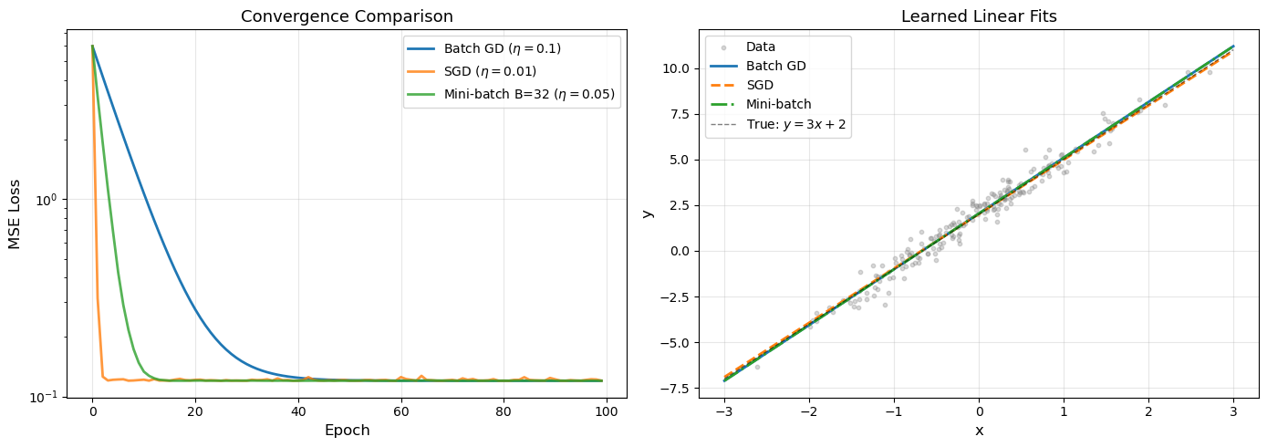
Batch GD:   w = [3.04999022 2.0448391 ] (true: [3, 2])
SGD:        w = [2.97109734 2.01201481] (true: [3, 2])
Mini-batch: w = [3.04952292 2.04253718] (true: [3, 2])
3D Loss Surface with Gradient Descent Trajectories#
The following visualization shows a 3D loss surface and gradient descent trajectories for different learning rates, providing geometric intuition for how the optimization proceeds.
Show code cell source
import numpy as np
import matplotlib.pyplot as plt
from mpl_toolkits.mplot3d import Axes3D

np.random.seed(42)

# Define loss surface: L(w1, w2) = w1^2 + 3*w2^2 + 0.5*sin(3*w1)*sin(3*w2)
def loss_surface(w1, w2):
    return w1**2 + 3*w2**2 + 0.5 * np.sin(3*w1) * np.sin(3*w2)

def loss_grad(w):
    w1, w2 = w
    dw1 = 2*w1 + 0.5 * 3 * np.cos(3*w1) * np.sin(3*w2)
    dw2 = 6*w2 + 0.5 * np.sin(3*w1) * 3 * np.cos(3*w2)
    return np.array([dw1, dw2])

# Create grid
w1_range = np.linspace(-3, 3, 200)
w2_range = np.linspace(-2, 2, 200)
W1, W2 = np.meshgrid(w1_range, w2_range)
Z = loss_surface(W1, W2)

# Run GD for different learning rates
etas_3d = [0.01, 0.05, 0.15]
colors_3d = ['blue', 'green', 'red']
labels_3d = ['$\\eta=0.01$ (slow)', '$\\eta=0.05$ (good)', '$\\eta=0.15$ (aggressive)']

trajectories_3d = []
for eta in etas_3d:
    w = np.array([2.5, 1.5])
    traj = [w.copy()]
    for _ in range(100):
        g = loss_grad(w)
        w = w - eta * g
        traj.append(w.copy())
        if np.linalg.norm(w) > 50:
            break
    trajectories_3d.append(np.array(traj))

# Create figure with 3D surface and 2D contour side by side
fig = plt.figure(figsize=(16, 7))

# 3D surface plot
ax1 = fig.add_subplot(121, projection='3d')
ax1.plot_surface(W1, W2, Z, cmap='viridis', alpha=0.6, edgecolor='none')

for traj, color, label in zip(trajectories_3d, colors_3d, labels_3d):
    z_traj = loss_surface(traj[:, 0], traj[:, 1])
    ax1.plot(traj[:, 0], traj[:, 1], z_traj, 'o-', color=color,
             markersize=3, linewidth=2, label=label, zorder=10)

ax1.set_xlabel('$w_1$', fontsize=11)
ax1.set_ylabel('$w_2$', fontsize=11)
ax1.set_zlabel('Loss', fontsize=11)
ax1.set_title('3D Loss Surface with GD Trajectories', fontsize=12)
ax1.view_init(elev=35, azim=-60)
ax1.legend(fontsize=8, loc='upper right')

# 2D contour view
ax2 = fig.add_subplot(122)
ax2.contour(W1, W2, Z, levels=30, cmap='viridis', alpha=0.6)
ax2.contourf(W1, W2, Z, levels=30, cmap='viridis', alpha=0.2)

for traj, color, label in zip(trajectories_3d, colors_3d, labels_3d):
    ax2.plot(traj[:, 0], traj[:, 1], 'o-', color=color,
             markersize=3, linewidth=1.5, label=label, alpha=0.9)

ax2.plot(0, 0, 'k*', markersize=15, label='Global minimum')
ax2.set_xlabel('$w_1$', fontsize=12)
ax2.set_ylabel('$w_2$', fontsize=12)
ax2.set_title('Contour View', fontsize=12)
ax2.legend(fontsize=9)
ax2.grid(True, alpha=0.2)

plt.tight_layout()
plt.savefig('gd_3d_surface.png', dpi=150, bbox_inches='tight')
plt.show()

for traj, label in zip(trajectories_3d, labels_3d):
    final_loss = loss_surface(traj[-1, 0], traj[-1, 1])
    print(f"{label}: final point = ({traj[-1, 0]:.4f}, {traj[-1, 1]:.4f}), loss = {final_loss:.6f}")
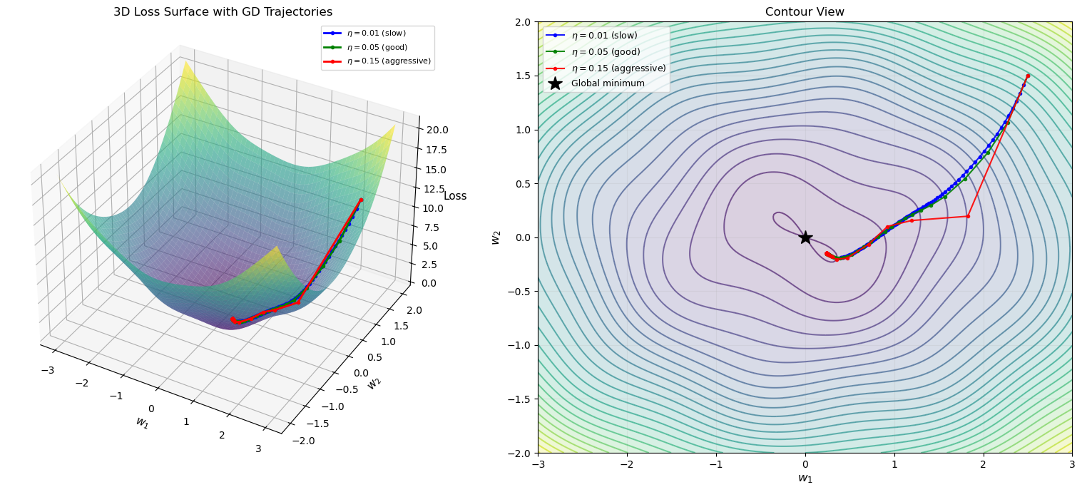
$\eta=0.01$ (slow): final point = (0.3988, -0.1887), loss = 0.016267
$\eta=0.05$ (good): final point = (0.2433, -0.1501), loss = -0.018322
$\eta=0.15$ (aggressive): final point = (0.2432, -0.1501), loss = -0.018322
Side-by-Side: Batch GD vs SGD vs Mini-batch Trajectories#
The following visualization shows the three optimization strategies on the same 2D loss surface, highlighting the key differences in their trajectories.
Show code cell source
import numpy as np
import matplotlib.pyplot as plt

np.random.seed(42)

# Loss surface: L(w1, w2) = w1^2 + 5*w2^2
def loss_fn(w):
    return w[0]**2 + 5*w[1]**2

def loss_grad_full(w):
    return np.array([2*w[0], 10*w[1]])

# Simulate noisy gradient (for SGD and mini-batch)
def loss_grad_noisy(w, noise_std=2.0):
    """Simulate stochastic gradient by adding noise to exact gradient."""
    g = loss_grad_full(w)
    return g + np.random.randn(2) * noise_std

def loss_grad_minibatch(w, noise_std=0.7):
    """Simulate mini-batch gradient (less noise than SGD)."""
    g = loss_grad_full(w)
    return g + np.random.randn(2) * noise_std

# Starting point
w0 = np.array([4.0, 2.0])
n_steps = 60

# Batch GD
w = w0.copy()
traj_batch = [w.copy()]
for _ in range(n_steps):
    w = w - 0.06 * loss_grad_full(w)
    traj_batch.append(w.copy())
traj_batch = np.array(traj_batch)

# SGD
np.random.seed(42)
w = w0.copy()
traj_sgd = [w.copy()]
for _ in range(n_steps):
    w = w - 0.04 * loss_grad_noisy(w, noise_std=3.0)
    traj_sgd.append(w.copy())
traj_sgd = np.array(traj_sgd)

# Mini-batch
np.random.seed(42)
w = w0.copy()
traj_mini = [w.copy()]
for _ in range(n_steps):
    w = w - 0.05 * loss_grad_minibatch(w, noise_std=1.0)
    traj_mini.append(w.copy())
traj_mini = np.array(traj_mini)

# Grid for contours
w1 = np.linspace(-5, 5, 200)
w2 = np.linspace(-3, 3, 200)
W1, W2 = np.meshgrid(w1, w2)
Z = W1**2 + 5*W2**2

# 3-panel plot
fig, axes = plt.subplots(1, 3, figsize=(18, 5))

titles = ['Batch GD (exact gradient)', 'SGD (single sample)', 'Mini-batch (B=32)']
trajs = [traj_batch, traj_sgd, traj_mini]
colors = ['blue', 'red', 'green']

for ax, traj, title, color in zip(axes, trajs, titles, colors):
    ax.contour(W1, W2, Z, levels=20, cmap='gray', alpha=0.4)
    ax.plot(traj[:, 0], traj[:, 1], 'o-', color=color, markersize=3,
            linewidth=1.2, alpha=0.8)
    ax.plot(traj[0, 0], traj[0, 1], 'ko', markersize=8, label='Start')
    ax.plot(0, 0, 'k*', markersize=15, label='Minimum')
    ax.set_xlabel('$w_1$', fontsize=12)
    ax.set_ylabel('$w_2$', fontsize=12)
    ax.set_title(title, fontsize=13)
    ax.legend(fontsize=9)
    ax.set_xlim(-5.5, 5.5)
    ax.set_ylim(-3.5, 3.5)
    ax.grid(True, alpha=0.2)
    ax.set_aspect('equal')

plt.suptitle('Comparison of Optimization Trajectories on $L = w_1^2 + 5w_2^2$',
             fontsize=14, fontweight='bold', y=1.02)
plt.tight_layout()
plt.savefig('gd_sgd_minibatch_comparison.png', dpi=150, bbox_inches='tight')
plt.show()

print("Notice:")
print("  - Batch GD: smooth, predictable path")
print("  - SGD: very noisy, zigzagging trajectory")
print("  - Mini-batch: moderate noise, good compromise")
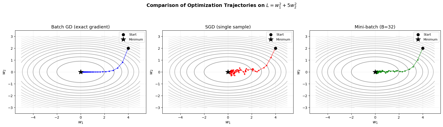
Notice:
  - Batch GD: smooth, predictable path
  - SGD: very noisy, zigzagging trajectory
  - Mini-batch: moderate noise, good compromise
Learning Rate Sweep Visualization#
The following plot shows loss curves for a range of learning rates on the same problem, clearly demonstrating how the learning rate affects convergence behavior.
Show code cell source
import numpy as np
import matplotlib.pyplot as plt

np.random.seed(42)

# Loss function: L(w) = w1^2 + 10*w2^2 (ill-conditioned quadratic)
def loss_fn(w):
    return w[0]**2 + 10*w[1]**2

def loss_grad(w):
    return np.array([2*w[0], 20*w[1]])

# Learning rate sweep
etas_sweep = [0.001, 0.01, 0.1, 1.0, 10.0]
w0 = np.array([4.0, 2.5])
n_iters = 100

fig, axes = plt.subplots(1, 2, figsize=(16, 6))

colors = ['#1f77b4', '#2ca02c', '#ff7f0e', '#d62728', '#9467bd']
styles = ['-', '-', '-', '--', ':']

for eta, color, style in zip(etas_sweep, colors, styles):
    w = w0.copy()
    losses = [loss_fn(w)]
    diverged = False
    for t in range(n_iters):
        g = loss_grad(w)
        w = w - eta * g
        l = loss_fn(w)
        if l > 1e10:
            losses.append(l)
            diverged = True
            break
        losses.append(l)

    label = f'$\\eta = {eta}$'
    if diverged:
        label += ' (DIVERGES)'

    axes[0].plot(losses, color=color, linewidth=2.5, linestyle=style, label=label)

axes[0].set_xlabel('Iteration', fontsize=13)
axes[0].set_ylabel('Loss $\\mathcal{L}(\\mathbf{w})$', fontsize=13)
axes[0].set_title('Learning Rate Sweep: Loss Curves', fontsize=14)
axes[0].set_yscale('log')
axes[0].set_ylim(1e-10, 1e12)
axes[0].legend(fontsize=11, loc='upper right')
axes[0].grid(True, alpha=0.3)
axes[0].axhline(y=1e-6, color='gray', linestyle=':', alpha=0.5, label='Convergence threshold')

# Convergence iteration bar chart (or infinity if diverged)
convergence_iters = []
threshold = 1e-4
for eta in etas_sweep:
    w = w0.copy()
    converged_at = n_iters
    for t in range(n_iters):
        g = loss_grad(w)
        w = w - eta * g
        if loss_fn(w) > 1e10:  # diverged
            converged_at = -1
            break
        if loss_fn(w) < threshold:
            converged_at = t + 1
            break
    convergence_iters.append(converged_at)

bar_colors = []
bar_vals = []
for ci, color in zip(convergence_iters, colors):
    bar_colors.append(color)
    bar_vals.append(ci if ci > 0 else n_iters)

bars = axes[1].bar(range(len(etas_sweep)), bar_vals, color=bar_colors, edgecolor='black')

# Mark diverged bars
for i, ci in enumerate(convergence_iters):
    if ci == -1:
        axes[1].text(i, bar_vals[i] + 1, 'DIVERGED', ha='center', fontsize=9,
                     color='red', fontweight='bold')
    elif ci == n_iters:
        axes[1].text(i, bar_vals[i] + 1, 'NOT\nCONVERGED', ha='center', fontsize=8,
                     color='orange')
    else:
        axes[1].text(i, bar_vals[i] + 1, f'{ci} iters', ha='center', fontsize=9)

axes[1].set_xticks(range(len(etas_sweep)))
axes[1].set_xticklabels([f'$\\eta={e}$' for e in etas_sweep], fontsize=10)
axes[1].set_xlabel('Learning Rate', fontsize=13)
axes[1].set_ylabel(f'Iterations to reach loss < {threshold}', fontsize=12)
axes[1].set_title('Convergence Speed vs Learning Rate', fontsize=14)
axes[1].grid(True, alpha=0.3, axis='y')

plt.tight_layout()
plt.savefig('learning_rate_sweep.png', dpi=150, bbox_inches='tight')
plt.show()

print("Summary of learning rate sweep:")
for eta, ci in zip(etas_sweep, convergence_iters):
    if ci == -1:
        print(f"  eta = {eta:6.3f}: DIVERGED")
    elif ci == n_iters:
        print(f"  eta = {eta:6.3f}: Did not converge in {n_iters} iterations")
    else:
        print(f"  eta = {eta:6.3f}: Converged in {ci} iterations")
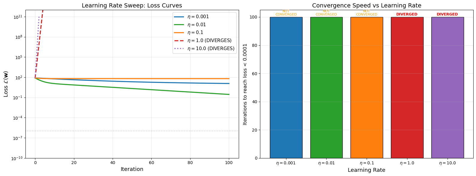
Summary of learning rate sweep:
  eta =  0.001: Did not converge in 100 iterations
  eta =  0.010: Did not converge in 100 iterations
  eta =  0.100: Did not converge in 100 iterations
  eta =  1.000: DIVERGED
  eta = 10.000: DIVERGED
15.8 Convergence Properties#
Batch Gradient Descent on Convex Functions#
For an \(L\)-smooth convex function with learning rate \(\eta \leq 1/L\):
For \(\mu\)-strongly convex functions (linear convergence):
The convergence rate depends on the condition number \(\kappa = L/\mu\).
SGD Convergence#
For SGD with diminishing learning rate \(\eta_t = \eta_0 / \sqrt{t}\) on convex functions:
where \(\bar{\mathbf{w}}_T\) is the average iterate. SGD is slower but cheaper per iteration.
Summary#
Method |
Cost per iter |
Convergence (convex) |
Convergence (strongly convex) |
|---|---|---|---|
Batch GD |
\(O(N)\) |
\(O(1/t)\) |
\(O(\rho^t)\) where \(\rho < 1\) |
SGD |
\(O(1)\) |
\(O(1/\sqrt{t})\) |
\(O(1/t)\) |
Mini-batch |
\(O(B)\) |
Between the two |
Between the two |
Exercises#
Exercise 15.1. Implement gradient descent with momentum: \(\mathbf{v}_{t+1} = \beta \mathbf{v}_t + \nabla \mathcal{L}(\mathbf{w}_t)\), \(\mathbf{w}_{t+1} = \mathbf{w}_t - \eta \mathbf{v}_{t+1}\). Compare trajectories on the quadratic bowl with and without momentum (\(\beta = 0.9\)).
Exercise 15.2. Prove that gradient descent on the quadratic \(\mathcal{L}(\mathbf{w}) = \frac{1}{2}\mathbf{w}^\top \mathbf{A}\mathbf{w} - \mathbf{b}^\top \mathbf{w}\) converges if and only if \(0 < \eta < 2/\lambda_{\max}(\mathbf{A})\).
Exercise 15.3. Implement a learning rate schedule: start with \(\eta_0 = 0.1\) and decay by a factor of 10 at epochs 50 and 80. Compare with constant learning rate on the MNIST-like spiral dataset.
Exercise 15.4. Generate a 1D non-convex function with multiple local minima. Run gradient descent from 20 different random initializations and plot where each one converges. What fraction find the global minimum?
Exercise 15.5. Derive the gradient of the cross-entropy loss combined with softmax. Show that \(\partial L / \partial z_j = \hat{y}_j - y_j\) where \(z_j\) are the logits.