Chapter 20: From McCulloch-Pitts to Backpropagation – The Complete Arc

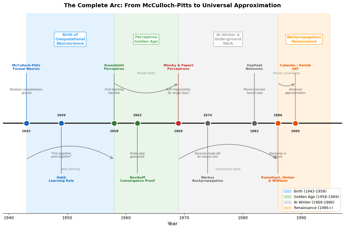
This final chapter synthesizes the journey we have taken through the classical foundations of neural networks. We trace the arc from McCulloch and Pitts’s formal neuron (1943) through Rosenblatt’s perceptron (1958), the downturn in neural network research associated with Minsky and Papert (1969), and the resurrection via backpropagation (1986), culminating in the Universal Approximation Theorem (1989). We identify the recurring themes, the key breakthroughs, and the obstacles that shaped the field.

Historical Perspective

The story of neural networks is one of the most dramatic in all of science. It spans nearly half a century of breakthroughs, setbacks, and comebacks – a narrative shaped as much by scientific politics and funding cycles as by theorems and algorithms. Understanding this history is not mere trivia: the patterns of hype, disappointment, and renewal continue to repeat in modern AI.

20.1 The Historical Timeline

Year	Milestone	Key Figure(s)	What Was Achieved
1943	McCulloch-Pitts neuron	McCulloch & Pitts	Formal model of a neuron; any Boolean function can be computed
1949	Hebbian learning	Donald Hebb	First learning rule: “neurons that fire together wire together”
1958	The Perceptron	Frank Rosenblatt	First machine that learns from data (perceptron convergence theorem)
1969	Perceptrons	Minsky & Papert	Proved linear separability limitations; triggered the AI winter
1974	Backpropagation	Paul Werbos	Applied reverse-mode automatic differentiation to neural networks
1982	Hopfield networks	John Hopfield	Revived interest in neural networks via physics connections
1986	Backprop popularized	Rumelhart, Hinton & Williams	Demonstrated that hidden layers could learn useful representations
1989	Universal Approximation	Hornik, Stinchcombe & White; Cybenko	Proved one hidden layer suffices for any continuous function

20.2 What Was Solved at Each Stage

1943: The Formal Neuron (McCulloch & Pitts)

Solved: How to model neural computation mathematically. Left open: How do the weights get set? (No learning rule.)

1949: Hebbian Learning (Hebb)

Solved: A biologically plausible principle for synaptic modification. Left open: How to use it for specific tasks? Stability? Multi-layer learning?

1958: The Perceptron (Rosenblatt)

Solved: A concrete learning algorithm with convergence guarantee. Left open: Only single-layer networks. What about non-linearly-separable problems?

1969: The Limitations (Minsky & Papert)

Solved (in a negative sense): Proved that single-layer perceptrons cannot compute XOR, parity, or connectivity. Established rigorous limits of linear classifiers. Left open: Can multi-layer networks overcome these limits? How to train them?

1974/1986: Backpropagation (Werbos / Rumelhart-Hinton-Williams)

Solved: The credit assignment problem. Efficient gradient computation for multi-layer networks. Demonstrated that hidden layers learn useful internal representations. Left open: Why is this so hard to train deep networks? Can networks approximate anything?

1989: Universal Approximation (Hornik et al. / Cybenko)

Solved: Neural networks are universal function approximators. Left open: Practical training of deep networks. Generalization. Efficiency.

Tip

Key Takeaway: 1943–1958 – The Birth of Computational Neuroscience

This era established the radical idea that the brain’s computation can be formalized mathematically. McCulloch and Pitts showed what neurons can compute (any Boolean function), and Hebb proposed how they might learn (correlation-based synaptic modification). The gap between these two – a computable model with no learning, and a learning principle with no concrete algorithm – would drive the next decade of research.

Tip

Key Takeaway: 1958–1969 – The Perceptron Golden Age

Rosenblatt’s perceptron bridged the gap: a concrete algorithm that provably learns from data. The convergence theorem gave mathematical certainty. But the excitement outpaced the reality – the perceptron could only learn linearly separable functions, and the media hype (“the embryo of an electronic computer that the Navy expects will be able to walk, talk, see, write, reproduce itself and be conscious of its existence”) set the stage for a devastating backlash.

Tip

Key Takeaway: 1969–1986 – The AI Winter and Underground Work

The Minsky-Papert book did not just prove a theorem – it changed the sociology of an entire field. Funding dried up, researchers moved to other areas, and neural networks became unfashionable. But crucial work continued underground: Werbos developed backpropagation (1974), Hopfield connected neural networks to physics (1982), and scattered researchers kept the flame alive. The lesson: important ideas can survive decades of neglect if a few committed researchers persist.

Tip

Key Takeaway: 1986+ – The Backpropagation Renaissance

Rumelhart, Hinton, and Williams did not just present an algorithm – they demonstrated empirically that multi-layer networks could learn meaningful internal representations. Combined with the Universal Approximation Theorem (1989), this provided both the tool (backprop) and the theoretical guarantee (UAT) that the tool was powerful enough. The lesson: a breakthrough needs both an algorithm that works in practice and a theory that explains why.

20.3 The Recurring Themes

Three themes recur throughout the entire history:

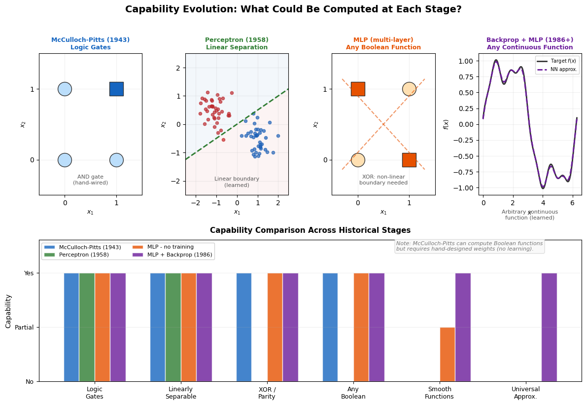
1. Representation

What can a network compute?

• McCulloch-Pitts: Any Boolean function (with hand-set weights)

• Perceptron: Linearly separable functions only

• MLP: Any continuous function (UAT)

2. Learning

How does a network acquire its computation?

• McCulloch-Pitts: No learning (weights fixed by design)

• Hebb: Unsupervised correlation-based learning

• Perceptron: Supervised, single-layer learning with convergence guarantee

• Backpropagation: Supervised, multi-layer learning via gradient descent

3. Universality

Are there fundamental limits?

• Perceptron: Yes – linear separability barrier

• MLP with backprop: Representationally universal (UAT)

• In practice: Depth matters, optimization is hard, generalization is subtle

Historical Reflection: The Sociology of Science

The history of neural networks teaches us that scientific progress is not purely a function of ideas and evidence. Funding, fashion, and personalities play enormous roles. Minsky’s outsized influence at MIT was as important as his mathematics in shaping the AI winter. Hinton’s persistence during the dark years was as important as backpropagation itself in enabling the revival. Students of science should study not just the theorems, but the humans who proved (or failed to prove) them.

20.4 Side-by-Side Comparison

Property	M-P Neuron (1943)	Perceptron (1958)	MLP + Backprop (1986)
Architecture	Single threshold unit	Single layer	Multiple layers
Activation	Binary step	Binary step	Sigmoid (later ReLU)
Learning	None	Perceptron rule	Backpropagation
Can learn?	No	Yes (linearly separable)	Can approximate any continuous function on compact domains, in principle
XOR?	Yes (manual)	No	Yes
Theory	Boolean completeness	Convergence theorem	Universal approximation
Biological basis	High	Moderate	Low
Parameters	Hand-designed	Learned (single layer)	Learned (all layers)
Key limitation	No learning	Linear separability	Vanishing gradient (for sigmoid)

20.5 The Three Key Breakthroughs

Breakthrough 1: The Formal Neuron (1943)

McCulloch and Pitts showed that neural computation could be formalized mathematically. This was the foundational insight: the brain’s computation can be modeled, analyzed, and potentially replicated.

Impact: Created the field of computational neuroscience and inspired AI.

Breakthrough 2: Learning Algorithms (1958)

Rosenblatt’s perceptron showed that machines could learn from examples. The convergence theorem provided the first mathematical guarantee for a learning algorithm.

Impact: Demonstrated that learning – not just computation – could be automated.

Breakthrough 3: Deep Learning via Backpropagation (1986)

Rumelhart, Hinton, and Williams showed that hidden-layer representations could be learned automatically. Backpropagation solved the credit assignment problem.

Impact: Enabled the training of multi-layer networks, overcoming the linear separability barrier and eventually leading to the deep learning revolution.

Danger

Lessons from AI Winters That Are STILL Relevant Today

The AI winter of 1969–1986 was not just a historical curiosity. Its causes are structural and recurring:

1. Overpromising capabilities leads to backlash. Rosenblatt and the media promised machines that could “see, walk, talk, and be conscious.” When the perceptron could not even learn XOR, the disillusionment was proportional to the hype. Today’s claims about AGI invite the same risk.

2. A single negative result can derail an entire field. Minsky and Papert’s book proved a narrow result (limitations of single-layer perceptrons), but it was widely interpreted as proving neural networks were fundamentally flawed. One influential critique, amplified by institutional power, froze a generation of research.

3. Fundamental advances often come from revisiting “dead” ideas. Backpropagation was essentially reverse-mode automatic differentiation applied to neural networks – an idea that could have been developed decades earlier. The key insight (Werbos, 1974) came from someone willing to work on an “unfashionable” topic.

4. The gap between “existence proof” and “practical algorithm” can be decades. Everyone knew multi-layer networks could solve XOR. But without a training algorithm, that knowledge was useless. The UAT (1989) proved universality, but practical deep learning took another 20+ years.

Warning

History Repeats: The Current AI Hype Cycle Has Parallels to the 1960s

Consider the parallels:

1960s	2020s
“The perceptron will be conscious”	“AGI is 2–5 years away”
Media amplifies modest results	Media amplifies benchmark scores
Funding pours into a narrow approach	Billions flow into scaling LLMs
Fundamental limitations ignored	Hallucination, reasoning limits ignored
One negative result triggers winter	What will be this era’s Perceptrons book?

This is not to say current AI is overhyped – the capabilities are genuinely remarkable. But the pattern of hype-backlash-winter is a sociological dynamic that operates independently of technical merit. Wise practitioners manage expectations carefully.

20.6 The Three Key Obstacles

Obstacle 1: No Learning Mechanism (1943–1958)

McCulloch-Pitts neurons could compute but not learn. Weights had to be set by hand.

Solved by: Rosenblatt’s perceptron learning rule (1958).

Obstacle 2: Linear Separability Barrier (1958–1986)

Minsky and Papert proved that single-layer perceptrons cannot learn non-linearly-separable functions. Hidden layers were needed but could not be trained.

Solved by: Multi-layer networks trained with backpropagation (1986).

Obstacle 3: Credit Assignment Problem (1969–1986)

Given an error at the output, how do we determine which hidden-layer weights are responsible?

Solved by: Backpropagation (chain rule applied to compute exact gradients through all layers).

Historical Reflection: The Unsung Heroes

The standard narrative credits McCulloch-Pitts, Rosenblatt, and Rumelhart-Hinton-Williams. But several crucial contributors are often overlooked:

• Paul Werbos (1974) developed backpropagation in his PhD thesis – 12 years before RHW’s famous Nature paper. He did this during the AI winter, when neural networks were considered a dead end.

• Seppo Linnainmaa (1970) invented reverse-mode automatic differentiation – the mathematical foundation of backpropagation – as part of his Master’s thesis.

• John Hopfield (1982) revived interest in neural networks from outside the AI community, using physics (energy functions, Boltzmann distributions) to make neural networks respectable again.

• Yann LeCun (1985) independently developed backpropagation in France, before the RHW paper.

The lesson: breakthroughs often have multiple independent discoverers, and priority does not always go to the first but to the most effectively communicated.

20.7 What Comes Next

The classical foundations covered in this course (1943–1989) established the core principles. The modern era builds upon them:

Convolutional Neural Networks (CNNs)

• LeCun et al. (1989): LeNet for handwritten digit recognition

• Krizhevsky et al. (2012): AlexNet – the deep learning revolution in computer vision

• Key idea: weight sharing exploits spatial structure

Recurrent Neural Networks (RNNs)

• Elman (1990), Jordan (1986): Processing sequences

• Backpropagation through time (BPTT)

• Key idea: shared weights across time steps

Long Short-Term Memory (LSTM)

• Hochreiter & Schmidhuber (1997)

• Solved the vanishing gradient problem for sequences

• Key idea: gated memory cells

Attention and Transformers

• Bahdanau et al. (2014): Attention mechanism

• Vaswani et al. (2017): “Attention Is All You Need” – the Transformer

• Key idea: self-attention replaces recurrence with parallel computation

• Foundation of GPT, BERT, and modern large language models

All of these architectures rely on the same core machinery: parameterized differentiable functions trained by gradient descent via backpropagation.

Historical Reflection: The Long Road from Theory to Practice

Consider the timeline from theoretical possibility to practical impact:

• 1943: McCulloch-Pitts prove Boolean completeness.

  • Time to practical learning: 15 years (perceptron, 1958).

• 1969: Everyone knows multi-layer networks can solve XOR.

  • Time to practical training: 17 years (backpropagation popularized, 1986).

• 1989: Universal Approximation Theorem proved.

  • Time to practical deep learning: 23 years (AlexNet, 2012).

Knowing something is possible and knowing how to do it efficiently are very different. The gap is always filled by engineering, hardware, data, and persistence.

Show code cell source Hide code cell source

import numpy as np
import matplotlib.pyplot as plt

# ============================================================
# Final Comprehensive Demo: Two Moons Classification
# ============================================================

np.random.seed(42)

def make_moons(n_samples=500, noise=0.1):
    """Generate two-moons dataset."""
    n = n_samples // 2
    # Upper moon
    theta1 = np.linspace(0, np.pi, n)
    x1 = np.cos(theta1) + np.random.randn(n) * noise
    y1 = np.sin(theta1) + np.random.randn(n) * noise
    # Lower moon (shifted)
    theta2 = np.linspace(0, np.pi, n)
    x2 = 1 - np.cos(theta2) + np.random.randn(n) * noise
    y2 = 1 - np.sin(theta2) - 0.5 + np.random.randn(n) * noise
    
    X = np.vstack([np.hstack([x1, x2]), np.hstack([y1, y2])])
    Y = np.hstack([np.zeros(n), np.ones(n)]).reshape(1, -1)
    return X, Y

X_moons, Y_moons = make_moons(n_samples=600, noise=0.15)

# Build a Neural Network (reusing the class from Chapter 18)
class NeuralNetwork:
    def __init__(self, layer_sizes, activation='sigmoid'):
        self.layer_sizes = layer_sizes
        self.L = len(layer_sizes) - 1
        self.activation_name = activation
        self.weights = []
        self.biases = []
        for l in range(self.L):
            n_in, n_out = layer_sizes[l], layer_sizes[l+1]
            W = np.random.randn(n_out, n_in) * np.sqrt(2.0 / (n_in + n_out))
            b = np.zeros((n_out, 1))
            self.weights.append(W)
            self.biases.append(b)
        self.z_cache = []
        self.a_cache = []
    
    def _activation(self, z):
        if self.activation_name == 'sigmoid':
            return 1.0 / (1.0 + np.exp(-np.clip(z, -500, 500)))
        elif self.activation_name == 'relu':
            return np.maximum(0, z)
    
    def _activation_derivative(self, z):
        if self.activation_name == 'sigmoid':
            s = self._activation(z)
            return s * (1 - s)
        elif self.activation_name == 'relu':
            return (z > 0).astype(float)
    
    def forward(self, X):
        self.z_cache = []
        self.a_cache = [X]
        a = X
        for l in range(self.L):
            z = self.weights[l] @ a + self.biases[l]
            a = self._activation(z)
            self.z_cache.append(z)
            self.a_cache.append(a)
        return a
    
    def compute_loss(self, y_hat, Y):
        m = Y.shape[1]
        return 0.5 * np.sum((y_hat - Y)**2) / m
    
    def backward(self, Y):
        m = Y.shape[1]
        dW = [None] * self.L
        db = [None] * self.L
        a_L = self.a_cache[-1]
        dL_da = (a_L - Y) / m
        sigma_prime = self._activation_derivative(self.z_cache[-1])
        delta = dL_da * sigma_prime
        dW[-1] = delta @ self.a_cache[-2].T
        db[-1] = np.sum(delta, axis=1, keepdims=True)
        for l in range(self.L - 2, -1, -1):
            sigma_prime = self._activation_derivative(self.z_cache[l])
            delta = (self.weights[l+1].T @ delta) * sigma_prime
            dW[l] = delta @ self.a_cache[l].T
            db[l] = np.sum(delta, axis=1, keepdims=True)
        return dW, db
    
    def train(self, X, Y, epochs, eta, verbose=True):
        losses = []
        for epoch in range(epochs):
            y_hat = self.forward(X)
            loss = self.compute_loss(y_hat, Y)
            losses.append(loss)
            dW, db = self.backward(Y)
            for l in range(self.L):
                self.weights[l] -= eta * dW[l]
                self.biases[l] -= eta * db[l]
            if verbose and (epoch % 500 == 0 or epoch == epochs - 1):
                print(f"Epoch {epoch:5d}: Loss = {loss:.6f}")
        return losses

# Train on two-moons
print("Training a 2-16-8-1 network on the two-moons dataset...\n")
nn = NeuralNetwork([2, 16, 8, 1], activation='sigmoid')
losses = nn.train(X_moons, Y_moons, epochs=5000, eta=5.0)

# Compute accuracy
y_pred = nn.forward(X_moons)
accuracy = np.mean((y_pred > 0.5).astype(float) == Y_moons)
print(f"\nFinal accuracy: {accuracy*100:.1f}%")

Training a 2-16-8-1 network on the two-moons dataset...

Epoch     0: Loss = 0.127298
Epoch   500: Loss = 0.042102

Epoch  1000: Loss = 0.035659
Epoch  1500: Loss = 0.005841

Epoch  2000: Loss = 0.003904
Epoch  2500: Loss = 0.003307

Epoch  3000: Loss = 0.003032
Epoch  3500: Loss = 0.002876

Epoch  4000: Loss = 0.002775
Epoch  4500: Loss = 0.002703

Epoch  4999: Loss = 0.002649

Final accuracy: 99.3%

Show code cell source Hide code cell source

# Visualization: Decision Boundary + Hidden Representations + Timeline

fig, axes = plt.subplots(2, 2, figsize=(16, 14))

# (1) Training loss
axes[0, 0].plot(losses, linewidth=2, color='navy')
axes[0, 0].set_xlabel('Epoch', fontsize=12)
axes[0, 0].set_ylabel('MSE Loss', fontsize=12)
axes[0, 0].set_title('Training Loss', fontsize=13)
axes[0, 0].set_yscale('log')
axes[0, 0].grid(True, alpha=0.3)

# (2) Decision boundary
xx, yy = np.meshgrid(np.linspace(-1.5, 2.5, 300), np.linspace(-1.5, 2.0, 300))
grid = np.c_[xx.ravel(), yy.ravel()].T
z_grid = nn.forward(grid).reshape(xx.shape)

axes[0, 1].contourf(xx, yy, z_grid, levels=50, cmap='RdBu_r', alpha=0.8)
axes[0, 1].contour(xx, yy, z_grid, levels=[0.5], colors='black', linewidths=2)
colors = ['red' if y == 0 else 'blue' for y in Y_moons[0]]
axes[0, 1].scatter(X_moons[0], X_moons[1], c=colors, s=10, alpha=0.5, edgecolors='none')
axes[0, 1].set_xlabel('$x_1$', fontsize=12)
axes[0, 1].set_ylabel('$x_2$', fontsize=12)
axes[0, 1].set_title('Learned Decision Boundary', fontsize=13)

# (3) Hidden layer representations (layer 1 activations)
_ = nn.forward(X_moons)  # populate cache
h1 = nn.a_cache[1]  # first hidden layer activations, shape (16, 600)

# Use first 2 hidden units for visualization
axes[1, 0].scatter(h1[0], h1[1], c=colors, s=10, alpha=0.5, edgecolors='none')
axes[1, 0].set_xlabel('Hidden unit 1', fontsize=12)
axes[1, 0].set_ylabel('Hidden unit 2', fontsize=12)
axes[1, 0].set_title('Hidden Layer 1 Representation (units 1 & 2)', fontsize=13)
axes[1, 0].grid(True, alpha=0.3)

# (4) Historical timeline
ax_timeline = axes[1, 1]
ax_timeline.set_xlim(1940, 2000)
ax_timeline.set_ylim(-1, 1)
ax_timeline.axhline(y=0, color='black', linewidth=2)

milestones = [
    (1943, 'McCulloch-\nPitts', 0.5),
    (1949, 'Hebb', -0.5),
    (1958, 'Perceptron', 0.5),
    (1969, 'Minsky-\nPapert', -0.5),
    (1974, 'Werbos\n(backprop)', 0.5),
    (1982, 'Hopfield', -0.5),
    (1986, 'RHW\n(backprop)', 0.5),
    (1989, 'UAT', -0.5),
]

for year, label, y_pos in milestones:
    color = 'green' if y_pos > 0 else 'darkorange'
    ax_timeline.plot(year, 0, 'o', color=color, markersize=10, zorder=5)
    ax_timeline.plot([year, year], [0, y_pos * 0.7], '-', color=color, linewidth=1.5)
    ax_timeline.text(year, y_pos * 0.85, label, ha='center', va='center', fontsize=9,
                     fontweight='bold', color=color)

# AI Winter shading
ax_timeline.axvspan(1969, 1982, alpha=0.1, color='blue', label='AI Winter')
ax_timeline.text(1975.5, 0.9, 'AI Winter', ha='center', fontsize=10, color='blue', style='italic')

ax_timeline.set_xlabel('Year', fontsize=12)
ax_timeline.set_title('The Complete Timeline: 1943-1989', fontsize=13)
ax_timeline.set_yticks([])
ax_timeline.grid(True, alpha=0.2, axis='x')

plt.suptitle('Chapter 20: From McCulloch-Pitts to Backpropagation',
             fontsize=15, fontweight='bold', y=1.01)
plt.tight_layout()
plt.savefig('synthesis_final.png', dpi=150, bbox_inches='tight')
plt.show()

Show code cell source Hide code cell source

import numpy as np
import matplotlib.pyplot as plt
import matplotlib.patches as mpatches
from matplotlib.patches import FancyArrowPatch

# ============================================================
# Complete Arc Diagram: The Full Neural Network Timeline
# Color-coded periods with key milestones and connecting arrows
# ============================================================

fig, ax = plt.subplots(figsize=(12, 8))

# Define eras with colors
eras = [
    (1943, 1958, 'Birth of\nComputational\nNeuroscience', '#2196F3', 0.12),
    (1958, 1969, 'Perceptron\nGolden Age', '#4CAF50', 0.12),
    (1969, 1986, 'AI Winter &\nUnderground\nWork', '#9E9E9E', 0.12),
    (1986, 1995, 'Backpropagation\nRenaissance', '#FF9800', 0.12),
]

# Draw era backgrounds
for start, end, label, color, alpha in eras:
    ax.axvspan(start, end, alpha=alpha, color=color, zorder=0)
    mid = (start + end) / 2
    ax.text(mid, 9.2, label, ha='center', va='center', fontsize=9,
            fontweight='bold', color=color, alpha=0.9,
            bbox=dict(boxstyle='round,pad=0.3', facecolor='white', edgecolor=color, alpha=0.9))

# Main timeline axis
ax.axhline(y=5, color='#333333', linewidth=3, zorder=2)

# Milestones: (year, label, y_offset_direction, description, color)
milestones = [
    (1943, 'McCulloch-Pitts\nFormal Neuron', 1, 'Boolean completeness\nproved', '#1565C0'),
    (1949, 'Hebb\nLearning Rule', -1, '"Fire together,\nwire together"', '#1565C0'),
    (1958, 'Rosenblatt\nPerceptron', 1, 'First learning\nmachine', '#2E7D32'),
    (1962, 'Novikoff\nConvergence Proof', -1, 'Finite-step\nguarantee', '#2E7D32'),
    (1969, 'Minsky & Papert\nPerceptrons', 1, 'XOR impossibility\nfor single layer', '#C62828'),
    (1974, 'Werbos\nBackpropagation', -1, 'Reverse-mode AD\nfor neural nets', '#616161'),
    (1982, 'Hopfield\nNetworks', 1, 'Physics revives\nneural nets', '#616161'),
    (1986, 'Rumelhart, Hinton\n& Williams', -1, 'Backprop in\nNature', '#E65100'),
    (1989, 'Cybenko / Hornik\nUAT', 1, 'Universal\napproximation', '#E65100'),
]

for i, (year, label, direction, desc, color) in enumerate(milestones):
    y_dot = 5
    y_label = 5 + direction * 2.8
    y_desc = 5 + direction * 1.6
    
    # Milestone dot
    ax.plot(year, y_dot, 'o', color=color, markersize=14, zorder=5,
            markeredgecolor='white', markeredgewidth=2)
    
    # Connecting line
    ax.plot([year, year], [y_dot, y_label - direction * 0.3], '-',
            color=color, linewidth=1.5, zorder=3, alpha=0.7)
    
    # Year label
    ax.text(year, y_dot - direction * 0.4, str(year), ha='center', va='center',
            fontsize=8, fontweight='bold', color='#333333')
    
    # Milestone name
    ax.text(year, y_label, label, ha='center', va='center',
            fontsize=8, fontweight='bold', color=color)
    
    # Description
    ax.text(year, y_desc, desc, ha='center', va='center',
            fontsize=7, color='#555555', style='italic')

# Draw connecting arrows between key breakthroughs
arrow_connections = [
    (1943, 1958, 'Adds learning', 3.2),
    (1958, 1969, 'Proves limits', 7.0),
    (1969, 1986, 'Overcomes limits', 3.2),
    (1986, 1989, 'Proves universality', 7.0),
]

for start_yr, end_yr, label, y_arc in arrow_connections:
    mid = (start_yr + end_yr) / 2
    # Draw curved arrow
    arrow = FancyArrowPatch(
        (start_yr, y_arc), (end_yr, y_arc),
        connectionstyle=f'arc3,rad={0.3 if y_arc > 5 else -0.3}',
        arrowstyle='->', color='#888888', linewidth=1.5,
        mutation_scale=15, zorder=1
    )
    ax.add_patch(arrow)
    # Arrow label
    y_text = y_arc + (0.5 if y_arc > 5 else -0.5)
    ax.text(mid, y_text, label, ha='center', va='center',
            fontsize=7, color='#888888', style='italic')

# Formatting
ax.set_xlim(1939, 1997)
ax.set_ylim(0.5, 10.5)
ax.set_xlabel('Year', fontsize=12)
ax.set_yticks([])
ax.set_title('The Complete Arc: From McCulloch-Pitts to Universal Approximation',
             fontsize=14, fontweight='bold', pad=15)

# Legend
legend_patches = [
    mpatches.Patch(color='#2196F3', alpha=0.3, label='Birth (1943-1958)'),
    mpatches.Patch(color='#4CAF50', alpha=0.3, label='Golden Age (1958-1969)'),
    mpatches.Patch(color='#9E9E9E', alpha=0.3, label='AI Winter (1969-1986)'),
    mpatches.Patch(color='#FF9800', alpha=0.3, label='Renaissance (1986+)'),
]
ax.legend(handles=legend_patches, loc='lower right', fontsize=9,
          framealpha=0.9, edgecolor='#cccccc')

ax.spines['top'].set_visible(False)
ax.spines['right'].set_visible(False)
ax.spines['left'].set_visible(False)

plt.tight_layout()
plt.show()

Show code cell source Hide code cell source

import numpy as np
import matplotlib.pyplot as plt

# ============================================================
# Summary Table of ALL Key Results in the Book
# ============================================================

fig, ax = plt.subplots(figsize=(12, 8))
ax.axis('off')

# Table data
columns = ['Year', 'Author(s)', 'Result', 'Ch. Ref.', 'Significance']
data = [
    ['1943', 'McCulloch & Pitts', 'Formal neuron model', 'Ch. 1-3',
     'Any Boolean function computable'],
    ['1949', 'Hebb', 'Hebbian learning rule', 'Ch. 4-6',
     'First learning principle'],
    ['1958', 'Rosenblatt', 'Perceptron algorithm', 'Ch. 7-9',
     'First learning machine'],
    ['1962', 'Novikoff', 'Convergence theorem', 'Ch. 10',
     'Finite-step guarantee'],
    ['1969', 'Minsky & Papert', 'Linear separability limits', 'Ch. 11-12',
     'XOR impossibility (single layer)'],
    ['1970', 'Linnainmaa', 'Reverse-mode AD', 'Ch. 14',
     'Mathematical basis for backprop'],
    ['1974', 'Werbos', 'Backprop for neural nets', 'Ch. 14-15',
     'Credit assignment solved'],
    ['1982', 'Oja', 'PCA via Hebbian learning', 'Ch. 6',
     'Stabilized Hebb rule'],
    ['1982', 'Hopfield', 'Energy-based networks', 'Ch. 13',
     'Physics revives the field'],
    ['1986', 'Rumelhart et al.', 'Backprop popularized', 'Ch. 15-17',
     'Hidden representations learned'],
    ['1989', 'Cybenko', 'UAT (sigmoidal)', 'Ch. 18-19',
     'One hidden layer suffices'],
    ['1989', 'Hornik et al.', 'UAT (general)', 'Ch. 18-19',
     'Universal approximation proved'],
]

# Color rows by era
era_colors = {
    'birth': '#E3F2FD',       # blue - light
    'golden': '#E8F5E9',      # green - light
    'winter': '#F5F5F5',      # grey - light
    'renaissance': '#FFF3E0', # orange - light
}

row_colors = [
    era_colors['birth'],      # 1943 M-P
    era_colors['birth'],      # 1949 Hebb
    era_colors['golden'],     # 1958 Rosenblatt
    era_colors['golden'],     # 1962 Novikoff
    era_colors['winter'],     # 1969 M&P
    era_colors['winter'],     # 1970 Linnainmaa
    era_colors['winter'],     # 1974 Werbos
    era_colors['winter'],     # 1982 Oja
    era_colors['winter'],     # 1982 Hopfield
    era_colors['renaissance'],# 1986 RHW
    era_colors['renaissance'],# 1989 Cybenko
    era_colors['renaissance'],# 1989 Hornik
]

table = ax.table(
    cellText=data,
    colLabels=columns,
    cellLoc='center',
    loc='center',
    colWidths=[0.06, 0.16, 0.22, 0.08, 0.30]
)

# Style the table
table.auto_set_font_size(False)
table.set_fontsize(9)
table.scale(1.0, 1.8)

# Header styling
for j in range(len(columns)):
    cell = table[0, j]
    cell.set_facecolor('#37474F')
    cell.set_text_props(color='white', fontweight='bold', fontsize=10)

# Row styling
for i in range(len(data)):
    for j in range(len(columns)):
        cell = table[i + 1, j]
        cell.set_facecolor(row_colors[i])
        cell.set_edgecolor('#BDBDBD')
        if j == 0:  # Year column bold
            cell.set_text_props(fontweight='bold')

ax.set_title('Summary of Key Results Across All Chapters',
             fontsize=14, fontweight='bold', pad=20)

# Era legend below table
legend_text = ('Color coding:  '
               'Blue = Birth (1943-1958)  |  '
               'Green = Golden Age (1958-1969)  |  '
               'Grey = AI Winter (1969-1986)  |  '
               'Orange = Renaissance (1986+)')
fig.text(0.5, 0.02, legend_text, ha='center', fontsize=9, style='italic', color='#555555')

plt.tight_layout()
plt.show()

Show code cell source Hide code cell source

import numpy as np
import matplotlib.pyplot as plt
import matplotlib.patches as mpatches

# ============================================================
# Capability Evolution Plot
# What could be computed at each historical stage?
# ============================================================

np.random.seed(42)

fig, axes = plt.subplots(2, 4, figsize=(12, 8))

# ---- Top row: The function classes at each stage ----

# 1. McCulloch-Pitts: Logic gates (AND, OR, NOT)
ax = axes[0, 0]
ax.set_title('McCulloch-Pitts (1943)\nLogic Gates', fontsize=9, fontweight='bold',
             color='#1565C0')
# Draw AND gate truth table
inputs = [(0, 0), (0, 1), (1, 0), (1, 1)]
and_out = [0, 0, 0, 1]
for (x1, x2), y in zip(inputs, and_out):
    color = '#1565C0' if y == 1 else '#BBDEFB'
    marker = 's' if y == 1 else 'o'
    ax.plot(x1, x2, marker, color=color, markersize=20, markeredgecolor='#333')
ax.set_xlim(-0.5, 1.5)
ax.set_ylim(-0.5, 1.5)
ax.set_xlabel('$x_1$', fontsize=9)
ax.set_ylabel('$x_2$', fontsize=9)
ax.text(0.5, -0.35, 'AND gate\n(hand-wired)', ha='center', fontsize=8, color='#555')
ax.set_xticks([0, 1])
ax.set_yticks([0, 1])
ax.grid(True, alpha=0.2)

# 2. Perceptron: Linearly separable functions
ax = axes[0, 1]
ax.set_title('Perceptron (1958)\nLinear Separation', fontsize=9, fontweight='bold',
             color='#2E7D32')
# Generate linearly separable data
n_pts = 40
class0 = np.random.randn(2, n_pts) * 0.4 + np.array([[-1], [0.5]])
class1 = np.random.randn(2, n_pts) * 0.4 + np.array([[1], [-0.5]])
ax.scatter(class0[0], class0[1], c='#C62828', s=20, alpha=0.7, label='Class 0')
ax.scatter(class1[0], class1[1], c='#1565C0', s=20, alpha=0.7, label='Class 1')
x_line = np.linspace(-2.5, 2.5, 100)
ax.plot(x_line, x_line * 0.5, '--', color='#2E7D32', linewidth=2)
ax.fill_between(x_line, x_line * 0.5, 2.5, alpha=0.05, color='#1565C0')
ax.fill_between(x_line, -2.5, x_line * 0.5, alpha=0.05, color='#C62828')
ax.set_xlim(-2.5, 2.5)
ax.set_ylim(-2.5, 2.5)
ax.set_xlabel('$x_1$', fontsize=9)
ax.set_ylabel('$x_2$', fontsize=9)
ax.text(0, -2.2, 'Linear boundary\n(learned)', ha='center', fontsize=8, color='#555')
ax.grid(True, alpha=0.2)

# 3. MLP: Any Boolean function (XOR)
ax = axes[0, 2]
ax.set_title('MLP (multi-layer)\nAny Boolean Function', fontsize=9, fontweight='bold',
             color='#E65100')
# XOR
xor_inputs = [(0, 0), (0, 1), (1, 0), (1, 1)]
xor_out = [0, 1, 1, 0]
for (x1, x2), y in zip(xor_inputs, xor_out):
    color = '#E65100' if y == 1 else '#FFE0B2'
    marker = 's' if y == 1 else 'o'
    ax.plot(x1, x2, marker, color=color, markersize=20, markeredgecolor='#333')
# Draw XOR boundary (two lines)
x_line = np.linspace(-0.3, 1.3, 100)
ax.plot(x_line, 0.5 + 0.8 * (x_line - 0.5), '--', color='#E65100', linewidth=1.5, alpha=0.6)
ax.plot(x_line, 0.5 - 0.8 * (x_line - 0.5), '--', color='#E65100', linewidth=1.5, alpha=0.6)
ax.set_xlim(-0.5, 1.5)
ax.set_ylim(-0.5, 1.5)
ax.set_xlabel('$x_1$', fontsize=9)
ax.set_ylabel('$x_2$', fontsize=9)
ax.text(0.5, -0.35, 'XOR: non-linear\nboundary needed', ha='center', fontsize=8, color='#555')
ax.set_xticks([0, 1])
ax.set_yticks([0, 1])
ax.grid(True, alpha=0.2)

# 4. Backprop + MLP: Any continuous function (UAT)
ax = axes[0, 3]
ax.set_title('Backprop + MLP (1986+)\nAny Continuous Function', fontsize=9,
             fontweight='bold', color='#6A1B9A')
# Show a complex 1D function and its neural net approximation
x_func = np.linspace(0, 2 * np.pi, 200)
y_target = np.sin(x_func) + 0.3 * np.sin(3 * x_func) + 0.1 * np.cos(7 * x_func)
# Simulate a neural net approximation (smooth version)
y_approx = np.sin(x_func) + 0.28 * np.sin(3 * x_func) + 0.08 * np.cos(7 * x_func)
ax.plot(x_func, y_target, '-', color='#333333', linewidth=2, label='Target $f(x)$')
ax.plot(x_func, y_approx, '--', color='#6A1B9A', linewidth=2, label='NN approx.')
ax.fill_between(x_func, y_target, y_approx, alpha=0.15, color='#6A1B9A')
ax.set_xlabel('$x$', fontsize=9)
ax.set_ylabel('$f(x)$', fontsize=9)
ax.text(np.pi, -1.5, 'Arbitrary continuous\nfunction (learned)', ha='center',
        fontsize=8, color='#555')
ax.legend(fontsize=7, loc='upper right')
ax.grid(True, alpha=0.2)

# ---- Bottom row: Capability summary bar chart ----

# Merge bottom 4 axes into one
for a in axes[1, :]:
    a.remove()
ax_bottom = fig.add_subplot(2, 1, 2)

# Capability categories
categories = ['Logic\nGates', 'Linearly\nSeparable', 'XOR /\nParity', 'Any\nBoolean',
              'Smooth\nFunctions', 'Universal\nApprox.']
n_cat = len(categories)

# Models and their capabilities (1 = yes, 0 = no, 0.5 = partial)
models = {
    'McCulloch-Pitts (1943)': [1, 1, 1, 1, 0, 0],
    'Perceptron (1958)':      [1, 1, 0, 0, 0, 0],
    'MLP - no training':      [1, 1, 1, 1, 0.5, 0],
    'MLP + Backprop (1986)':  [1, 1, 1, 1, 1, 1],
}

model_colors = ['#1565C0', '#2E7D32', '#E65100', '#6A1B9A']
bar_width = 0.18
x_pos = np.arange(n_cat)

for i, (model_name, caps) in enumerate(models.items()):
    offset = (i - 1.5) * bar_width
    bars = ax_bottom.bar(x_pos + offset, caps, bar_width, label=model_name,
                         color=model_colors[i], alpha=0.8, edgecolor='white')

ax_bottom.set_xticks(x_pos)
ax_bottom.set_xticklabels(categories, fontsize=9)
ax_bottom.set_ylabel('Capability', fontsize=10)
ax_bottom.set_yticks([0, 0.5, 1])
ax_bottom.set_yticklabels(['No', 'Partial', 'Yes'], fontsize=9)
ax_bottom.set_ylim(0, 1.3)
ax_bottom.legend(fontsize=8, loc='upper left', ncol=2, framealpha=0.9)
ax_bottom.grid(True, alpha=0.2, axis='y')
ax_bottom.set_title('Capability Comparison Across Historical Stages', fontsize=11,
                     fontweight='bold', pad=10)

# Note about M-P
ax_bottom.text(3.5, 1.2, 'Note: McCulloch-Pitts can compute Boolean functions\n'
               'but requires hand-designed weights (no learning).',
               fontsize=8, style='italic', color='#777',
               bbox=dict(boxstyle='round', facecolor='#f9f9f9', edgecolor='#ddd'))

plt.suptitle('Capability Evolution: What Could Be Computed at Each Stage?',
             fontsize=14, fontweight='bold', y=1.02)
plt.tight_layout()
plt.show()

20.8 Reflection Questions

1. Why did it take 17 years from the Minsky-Papert critique (1969) to the backpropagation renaissance (1986)? What sociological and scientific factors contributed to the delay?

2. Biological plausibility vs. engineering utility: Hebbian learning is biologically plausible but limited. Backpropagation is powerful but biologically implausible. What does this tension tell us about the relationship between neuroscience and AI?

3. The role of proofs: How important were the formal proofs (perceptron convergence, Minsky-Papert impossibility, universal approximation) in shaping the field’s direction? Could the field have progressed faster with more or fewer theoretical results?

4. Depth vs. width: The Universal Approximation Theorem guarantees that width alone suffices. Yet modern practice favors deep, narrow networks over wide, shallow ones. Why? What does this say about the gap between existence proofs and practical algorithms?

5. Looking forward: Which of the unsolved problems from the classical era (generalization, efficiency, biological plausibility) do you think is most important for the future of AI?

6. The credit assignment problem revisited: Backpropagation solves credit assignment computationally. But does the brain solve the same problem? If so, how? If not, what problem does it solve instead?

Final Reflection: The Arc of Understanding

We began this course with a question: Can the brain’s computation be formalized? McCulloch and Pitts answered yes, in 1943. Each subsequent decade added another piece: learning (Hebb, Rosenblatt), the understanding of limits (Minsky-Papert), the ability to train deep networks (Werbos, Rumelhart-Hinton-Williams), and the proof of universality (Cybenko, Hornik).

The full arc – from formal neuron to universal approximator – took 46 years. It required mathematicians, psychologists, physicists, and computer scientists. It survived two world wars’ aftermath, an AI winter, and the rise and fall of multiple competing paradigms. And it produced the theoretical foundation upon which all of modern deep learning rests.

That foundation – parameterized differentiable functions trained by gradient descent – is the subject of this course, and the starting point for everything that comes next.