Chapter 27: Momentum, RMSProp, and Adam#
The story of neural network optimization is one of incremental genius. For decades after Robbins and Monro (1951) introduced stochastic approximation, practitioners relied on vanilla stochastic gradient descent (SGD) — a method that, while theoretically sound, suffers from painfully slow convergence on the rugged loss landscapes of neural networks.
The breakthrough came in stages. Boris Polyak (1964) introduced momentum, drawing an analogy to a heavy ball rolling downhill. Yurii Nesterov (1983) refined this with a “lookahead” trick that improved convergence on convex problems. Decades later, as deep learning reignited interest in neural networks, a new family of adaptive learning rate methods emerged: AdaGrad (Duchi, Hazan & Singer, 2011), RMSProp (Tieleman & Hinton, 2012), and finally Adam (Kingma & Ba, 2014), which combined the best ideas of momentum and adaptive rates into what became the default optimizer for deep learning.
This chapter derives each method from first principles, proves key convergence results, and demonstrates the dramatic practical differences on neural network training.
import numpy as np
import matplotlib.pyplot as plt

# Reproducible random number generator
rng = np.random.default_rng(42)

# Standard color palette for this chapter
COLORS = {
    'SGD': '#dc2626',       # red
    'Momentum': '#d97706',  # amber
    'Nesterov': '#3b82f6',  # blue
    'RMSProp': '#059669',   # green
    'Adam': '#4f46e5',      # indigo
    'AdaGrad': '#9333ea',   # purple
}

print("Imports loaded. Color palette defined.")
print("Colors:", list(COLORS.keys()))
Imports loaded. Color palette defined.
Colors: ['SGD', 'Momentum', 'Nesterov', 'RMSProp', 'Adam', 'AdaGrad']
27.1 The Problem with Vanilla SGD#
Recall from Chapter 15 the basic gradient descent update rule:
where \(\eta > 0\) is the learning rate and \(\nabla L(\mathbf{w}_t)\) is the gradient of the loss with respect to the parameters. This rule dates back to Cauchy (1847) for deterministic optimization and to Robbins and Monro (1951) for the stochastic case, making it one of the oldest algorithms in machine learning.
Despite its simplicity and strong theoretical guarantees (convergence to a local minimum under mild conditions), vanilla SGD suffers from three fundamental problems in practice:
Problem 1: Slow progress on flat regions#
When the gradient is small (e.g., on plateaus of the loss surface), the update \(\eta \nabla L\) is tiny, and the optimizer makes almost no progress. This is especially problematic with sigmoid activations, where gradients can be exponentially small.
Problem 2: Oscillation in narrow valleys#
When the loss surface has very different curvatures in different directions — that is, when the Hessian \(\mathbf{H} = \nabla^2 L\) is ill-conditioned — SGD oscillates back and forth across the narrow direction while making slow progress along the valley.
Definition: Condition Number
The condition number of a symmetric positive-definite matrix \(\mathbf{A}\) is
where \(\lambda_{\max}\) and \(\lambda_{\min}\) are the largest and smallest eigenvalues. A condition number \(\kappa \gg 1\) means the Hessian is ill-conditioned and SGD will struggle. For the quadratic \(L(w_1, w_2) = w_1^2 + 50 w_2^2\), the Hessian is \(\mathrm{diag}(2, 100)\) with \(\kappa = 50\).
Problem 3: Learning rate sensitivity#
The learning rate \(\eta\) must be set carefully:
Too large: the optimizer overshoots and diverges.
Too small: convergence is painfully slow.
The optimal \(\eta\) depends on the curvature, which varies across the loss surface.
The fundamental insight that drives the rest of this chapter is: different parameters need different effective learning rates, and the optimizer should accumulate information from past gradients to make better update decisions.
Show code cell source
# Visualization: SGD trajectory on an ill-conditioned quadratic

import numpy as np
import matplotlib.pyplot as plt

def ill_conditioned_quadratic(w):
    """L(w1, w2) = w1^2 + 50*w2^2"""
    return w[0]**2 + 50.0 * w[1]**2

def grad_quadratic(w):
    """Gradient of L(w1, w2) = w1^2 + 50*w2^2"""
    return np.array([2.0 * w[0], 100.0 * w[1]])

# Run SGD on the ill-conditioned quadratic
w = np.array([5.0, 0.5])
eta = 0.015
trajectory = [w.copy()]

for _ in range(80):
    g = grad_quadratic(w)
    w = w - eta * g
    trajectory.append(w.copy())

trajectory = np.array(trajectory)

# Plot
fig, ax = plt.subplots(1, 1, figsize=(10, 6))

# Contour plot
w1_grid = np.linspace(-6, 6, 300)
w2_grid = np.linspace(-1.0, 1.0, 300)
W1, W2 = np.meshgrid(w1_grid, w2_grid)
Z = W1**2 + 50.0 * W2**2

levels = [0.5, 1, 2, 5, 10, 15, 20, 30, 50]
ax.contour(W1, W2, Z, levels=levels, colors='gray', alpha=0.5, linewidths=0.8)
ax.contourf(W1, W2, Z, levels=levels, cmap='Blues', alpha=0.15)

# Trajectory
ax.plot(trajectory[:, 0], trajectory[:, 1], 'o-', color=COLORS['SGD'],
        markersize=3, linewidth=1.2, label=f'SGD ($\\eta={eta}$)', zorder=5)
ax.plot(trajectory[0, 0], trajectory[0, 1], 's', color='black', markersize=10,
        zorder=6, label='Start')
ax.plot(0, 0, '*', color='gold', markersize=15, markeredgecolor='black',
        markeredgewidth=1, zorder=6, label='Minimum')

ax.set_xlabel('$w_1$', fontsize=13)
ax.set_ylabel('$w_2$', fontsize=13)
ax.set_title('Vanilla SGD on an Ill-Conditioned Quadratic: $L = w_1^2 + 50\\,w_2^2$ ($\\kappa = 50$)',
             fontsize=13)
ax.legend(fontsize=11, loc='upper right')
ax.set_xlim(-6, 6)
ax.set_ylim(-1.0, 1.0)
ax.set_aspect('auto')
ax.grid(True, alpha=0.2)

plt.tight_layout()
plt.show()

print(f"After {len(trajectory)-1} steps: w = ({trajectory[-1,0]:.4f}, {trajectory[-1,1]:.6f})")
print(f"Loss: {ill_conditioned_quadratic(trajectory[-1]):.6f}")
print(f"The zigzag pattern is caused by the condition number kappa = 50.")
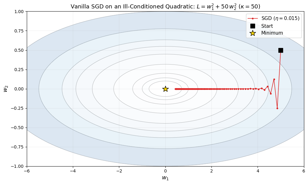
After 80 steps: w = (0.4372, 0.000000)
Loss: 0.191169
The zigzag pattern is caused by the condition number kappa = 50.
The plot above demonstrates the characteristic zigzag behavior of SGD on an ill-conditioned quadratic. The gradient in the \(w_2\) direction is 50 times stronger than in the \(w_1\) direction, so the optimizer oscillates violently in \(w_2\) while making slow progress in \(w_1\). Increasing the learning rate would speed up progress in \(w_1\) but would cause divergence in \(w_2\).
27.2 Momentum#
The key insight behind momentum is physical: imagine a heavy ball rolling down a hilly surface. The ball does not stop instantly when the slope becomes zero — its inertia carries it forward. Similarly, we can accumulate past gradients into a velocity vector that smooths out oscillations and accelerates progress along consistent gradient directions.
Definition: Momentum (Polyak, 1964)
The momentum update rule maintains a velocity vector \(\mathbf{v}_t\):
where \(\beta \in [0, 1)\) is the momentum coefficient (typically \(\beta = 0.9\)) and \(\mathbf{v}_0 = \mathbf{0}\).
Exponential moving average interpretation#
Unrolling the recurrence, we see that \(\mathbf{v}_{t+1}\) is an exponentially weighted sum of all past gradients:
The gradient from \(k\) steps ago is weighted by \(\beta^k\), so recent gradients contribute more. With \(\beta = 0.9\), a gradient from 10 steps ago has weight \(0.9^{10} \approx 0.35\), while one from 50 steps ago has weight \(0.9^{50} \approx 0.005\). Thus momentum effectively averages over a window of roughly \(\frac{1}{1-\beta} = 10\) gradients.
Why momentum helps#
Oscillation damping. In the \(w_2\) direction of our ill-conditioned quadratic, gradients alternate in sign. The velocity accumulates these alternating gradients, which partially cancel, reducing oscillation amplitude.
Acceleration along consistent directions. In the \(w_1\) direction, gradients consistently point toward the minimum. The velocity builds up, effectively increasing the learning rate in this direction.
Theorem: Momentum Convergence on Quadratics
For a quadratic objective \(L(\mathbf{w}) = \frac{1}{2}\mathbf{w}^T \mathbf{A} \mathbf{w}\) with \(\mathbf{A}\) symmetric positive definite, gradient descent with optimally tuned learning rate converges as:
while momentum with optimally tuned parameters \(\eta\) and \(\beta\) converges as:
where \(\kappa = \lambda_{\max} / \lambda_{\min}\) is the condition number.
Intuition: The convergence rate per step goes from \(\frac{\kappa-1}{\kappa+1}\) (close to 1 when \(\kappa\) is large) to \(\frac{\sqrt{\kappa}-1}{\sqrt{\kappa}+1}\). For \(\kappa = 100\): SGD rate \(= 0.98\), Momentum rate \(= 0.82\). This means momentum takes roughly \(\sqrt{\kappa}\) times fewer iterations. The optimal parameters are \(\eta^* = \left(\frac{2}{\sqrt{\lambda_{\max}} + \sqrt{\lambda_{\min}}}\right)^2\) and \(\beta^* = \left(\frac{\sqrt{\kappa}-1}{\sqrt{\kappa}+1}\right)^2\).
Nesterov Accelerated Gradient (NAG)#
Yurii Nesterov (1983) proposed a subtle but important modification: instead of evaluating the gradient at the current position \(\mathbf{w}_t\), evaluate it at the lookahead position \(\mathbf{w}_t - \eta \beta \mathbf{v}_t\) — the position where momentum alone would take us:
The intuition is: since we know momentum will carry us to \(\mathbf{w}_t - \eta \beta \mathbf{v}_t\), we might as well evaluate the gradient there and make a correction. This gives Nesterov momentum a “corrective” character that helps it slow down before overshooting.
# Momentum optimizer implementation

class MomentumOptimizer:
    """SGD with momentum (Polyak, 1964).

    Update rule:
        v_{t+1} = beta * v_t + grad
        w_{t+1} = w_t - eta * v_{t+1}
    """

    def __init__(self, eta=0.01, beta=0.9, nesterov=False):
        """
        Parameters
        ----------
        eta : float
            Learning rate.
        beta : float
            Momentum coefficient (typically 0.9).
        nesterov : bool
            If True, use Nesterov accelerated gradient.
        """
        self.eta = eta
        self.beta = beta
        self.nesterov = nesterov
        self.velocities = None  # initialized on first call

    def initialize(self, params):
        """Initialize velocity vectors to zeros matching param shapes."""
        self.velocities = [np.zeros_like(p) for p in params]

    def step(self, params, grads):
        """Perform one update step.

        Parameters
        ----------
        params : list of ndarray
            Current parameter values.
        grads : list of ndarray
            Gradients w.r.t. each parameter.

        Returns
        -------
        params : list of ndarray
            Updated parameters.
        """
        if self.velocities is None:
            self.initialize(params)

        updated = []
        for i, (p, g) in enumerate(zip(params, grads)):
            # Update velocity
            self.velocities[i] = self.beta * self.velocities[i] + g

            # Update parameter
            p_new = p - self.eta * self.velocities[i]
            updated.append(p_new)

        return updated


# Quick test on the quadratic
w = np.array([5.0, 0.5])
opt = MomentumOptimizer(eta=0.012, beta=0.9)
trajectory_mom = [w.copy()]

for _ in range(80):
    g = grad_quadratic(w)
    [w] = opt.step([w], [g])
    trajectory_mom.append(w.copy())

trajectory_mom = np.array(trajectory_mom)
print(f"Momentum optimizer defined.")
print(f"After 80 steps: w = ({trajectory_mom[-1,0]:.6f}, {trajectory_mom[-1,1]:.8f})")
print(f"Loss: {ill_conditioned_quadratic(trajectory_mom[-1]):.8f}")
Momentum optimizer defined.
After 80 steps: w = (0.052715, -0.00150814)
Loss: 0.00289262
Show code cell source
# Side-by-side comparison: SGD vs Momentum vs Nesterov on the ill-conditioned quadratic

import numpy as np
import matplotlib.pyplot as plt

def run_optimizer_quadratic(optimizer_type, w_init, eta, beta=0.9, n_steps=80):
    """Run an optimizer on L(w) = w1^2 + 50*w2^2."""
    w = w_init.copy()
    traj = [w.copy()]
    v = np.zeros_like(w)

    for _ in range(n_steps):
        if optimizer_type == 'sgd':
            g = grad_quadratic(w)
            w = w - eta * g
        elif optimizer_type == 'momentum':
            g = grad_quadratic(w)
            v = beta * v + g
            w = w - eta * v
        elif optimizer_type == 'nesterov':
            # Evaluate gradient at lookahead position
            w_lookahead = w - eta * beta * v
            g = grad_quadratic(w_lookahead)
            v = beta * v + g
            w = w - eta * v
        traj.append(w.copy())

    return np.array(traj)

w_init = np.array([5.0, 0.5])
eta = 0.012
n_steps = 80

traj_sgd = run_optimizer_quadratic('sgd', w_init, eta, n_steps=n_steps)
traj_mom = run_optimizer_quadratic('momentum', w_init, eta, beta=0.9, n_steps=n_steps)
traj_nes = run_optimizer_quadratic('nesterov', w_init, eta, beta=0.9, n_steps=n_steps)

# 3-panel plot
fig, axes = plt.subplots(1, 3, figsize=(18, 5))

w1_grid = np.linspace(-6, 6, 300)
w2_grid = np.linspace(-1.0, 1.0, 300)
W1, W2 = np.meshgrid(w1_grid, w2_grid)
Z = W1**2 + 50.0 * W2**2
levels = [0.5, 1, 2, 5, 10, 15, 20, 30, 50]

for ax, traj, name, color in [
    (axes[0], traj_sgd, 'SGD', COLORS['SGD']),
    (axes[1], traj_mom, 'Momentum ($\\beta=0.9$)', COLORS['Momentum']),
    (axes[2], traj_nes, 'Nesterov ($\\beta=0.9$)', COLORS['Nesterov']),
]:
    ax.contour(W1, W2, Z, levels=levels, colors='gray', alpha=0.5, linewidths=0.8)
    ax.contourf(W1, W2, Z, levels=levels, cmap='Blues', alpha=0.12)
    ax.plot(traj[:, 0], traj[:, 1], 'o-', color=color,
            markersize=2.5, linewidth=1.0, label=name)
    ax.plot(traj[0, 0], traj[0, 1], 's', color='black', markersize=8, zorder=6)
    ax.plot(0, 0, '*', color='gold', markersize=14, markeredgecolor='black',
            markeredgewidth=1, zorder=6)
    final_loss = ill_conditioned_quadratic(traj[-1])
    ax.set_title(f'{name}\nFinal loss: {final_loss:.4f}', fontsize=12)
    ax.set_xlabel('$w_1$', fontsize=12)
    ax.set_ylabel('$w_2$', fontsize=12)
    ax.set_xlim(-6, 6)
    ax.set_ylim(-1.0, 1.0)
    ax.grid(True, alpha=0.2)

plt.suptitle('Optimizer Trajectories on $L = w_1^2 + 50\\,w_2^2$ ($\\kappa = 50$, $\\eta = 0.012$, 80 steps)',
             fontsize=14, fontweight='bold', y=1.02)
plt.tight_layout(rect=[0, 0, 1, 0.92])
plt.show()

# Loss curves
fig, ax = plt.subplots(1, 1, figsize=(8, 5))
for traj, name, color in [
    (traj_sgd, 'SGD', COLORS['SGD']),
    (traj_mom, 'Momentum', COLORS['Momentum']),
    (traj_nes, 'Nesterov', COLORS['Nesterov']),
]:
    losses = [ill_conditioned_quadratic(w) for w in traj]
    ax.plot(losses, linewidth=2, color=color, label=name)

ax.set_xlabel('Step', fontsize=12)
ax.set_ylabel('Loss', fontsize=12)
ax.set_title('Convergence Comparison on Ill-Conditioned Quadratic', fontsize=13)
ax.set_yscale('log')
ax.legend(fontsize=11)
ax.grid(True, alpha=0.3)
plt.tight_layout()
plt.show()

print(f"Final losses after {n_steps} steps:")
print(f"  SGD:      {ill_conditioned_quadratic(traj_sgd[-1]):.6f}")
print(f"  Momentum: {ill_conditioned_quadratic(traj_mom[-1]):.6f}")
print(f"  Nesterov: {ill_conditioned_quadratic(traj_nes[-1]):.6f}")
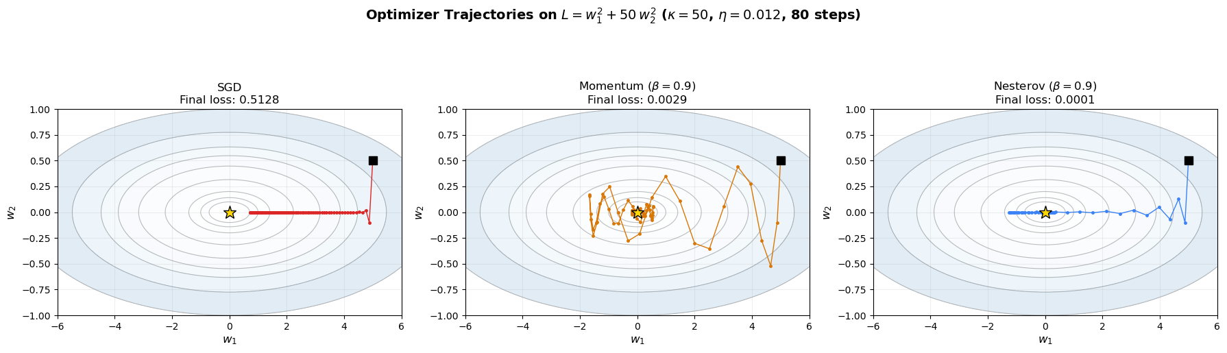

Final losses after 80 steps:
  SGD:      0.512756
  Momentum: 0.002893
  Nesterov: 0.000119
The plots above reveal the dramatic difference. SGD zigzags across the narrow valley, while momentum smooths out the oscillations and accelerates along the valley floor. Nesterov momentum is slightly more efficient — its “lookahead” correction helps it anticipate the curvature change and slow down appropriately.
Tip
Polyak’s momentum paper (1964) was published in the Soviet journal Zhurnal Vychislitel’noi Matematiki i Matematicheskoi Fiziki and remained largely unknown in the West for decades. Nesterov’s 1983 paper, which proved the \(O(\sqrt{\kappa})\) optimal convergence rate for convex optimization, is now considered one of the most important results in optimization theory.
27.3 Adaptive Learning Rates: AdaGrad and RMSProp#
Momentum addresses the oscillation problem by smoothing gradients over time, but it still uses a single global learning rate \(\eta\) for all parameters. A fundamentally different approach is to give each parameter its own adaptive learning rate based on the history of gradients for that parameter.
AdaGrad (Adaptive Gradient)#
Algorithm: AdaGrad (Duchi, Hazan & Singer, 2011)
Initialize: \(\mathbf{G}_0 = \mathbf{0}\) (accumulated squared gradients)
At each step \(t\):
Compute gradient: \(\mathbf{g}_t = \nabla L(\mathbf{w}_t)\)
Accumulate squared gradients: \(\mathbf{G}_t = \mathbf{G}_{t-1} + \mathbf{g}_t^2\) (element-wise)
Update: \(\mathbf{w}_{t+1} = \mathbf{w}_t - \dfrac{\eta}{\sqrt{\mathbf{G}_t + \epsilon}}\, \mathbf{g}_t\) (element-wise)
where \(\epsilon \approx 10^{-8}\) prevents division by zero.
The key idea: parameters with large accumulated gradients get smaller learning rates, and parameters with small accumulated gradients get larger learning rates. This is especially useful for sparse features (e.g., in natural language processing), where infrequent features need larger updates when they do appear.
Warning
AdaGrad’s fatal flaw: Since \(\mathbf{G}_t\) is a sum of squared gradients, it can only grow. Over time, the effective learning rate \(\eta / \sqrt{G_t}\) shrinks monotonically to zero, causing the optimizer to stop learning entirely. This makes AdaGrad unsuitable for non-convex problems like neural network training, where the optimizer must continue adapting throughout training.
RMSProp (Root Mean Square Propagation)#
Geoffrey Hinton’s fix for AdaGrad’s decaying learning rate is elegant: replace the ever-growing sum with an exponential moving average of squared gradients.
Algorithm: RMSProp (Tieleman & Hinton, 2012)
Initialize: \(\mathbf{v}_0 = \mathbf{0}\) (moving average of squared gradients)
At each step \(t\):
Compute gradient: \(\mathbf{g}_t = \nabla L(\mathbf{w}_t)\)
Update moving average: \(\mathbf{v}_t = \beta\, \mathbf{v}_{t-1} + (1-\beta)\, \mathbf{g}_t^2\) (element-wise)
Update: \(\mathbf{w}_{t+1} = \mathbf{w}_t - \dfrac{\eta}{\sqrt{\mathbf{v}_t + \epsilon}}\, \mathbf{g}_t\) (element-wise)
Typical hyperparameters: \(\beta = 0.9\), \(\eta = 0.001\), \(\epsilon = 10^{-8}\).
By using a moving average, RMSProp “forgets” old gradients and adapts to the recent gradient magnitudes. The denominator \(\sqrt{v_t}\) is an estimate of the root mean square of recent gradients, hence the name.
Tip
RMSProp is one of the most influential optimization ideas in deep learning history, yet it was never published as a paper. It first appeared as slide 29 of Lecture 6e in Geoffrey Hinton’s Coursera course “Neural Networks for Machine Learning” (2012). This makes it perhaps the most impactful unpublished result in machine learning.
# RMSProp optimizer implementation

class RMSPropOptimizer:
    """RMSProp optimizer (Tieleman & Hinton, 2012).

    Maintains an exponential moving average of squared gradients
    to adaptively scale the learning rate per parameter.

    Update rule:
        v_t = beta * v_{t-1} + (1 - beta) * g_t^2
        w_{t+1} = w_t - (eta / sqrt(v_t + eps)) * g_t
    """

    def __init__(self, eta=0.001, beta=0.99, epsilon=1e-8):
        """
        Parameters
        ----------
        eta : float
            Learning rate (default: 0.001).
        beta : float
            Decay rate for the moving average of squared gradients.
        epsilon : float
            Small constant for numerical stability.
        """
        self.eta = eta
        self.beta = beta
        self.epsilon = epsilon
        self.v = None  # moving average of squared gradients

    def initialize(self, params):
        """Initialize state to zeros matching param shapes."""
        self.v = [np.zeros_like(p) for p in params]

    def step(self, params, grads):
        """Perform one update step.

        Parameters
        ----------
        params : list of ndarray
            Current parameter values.
        grads : list of ndarray
            Gradients w.r.t. each parameter.

        Returns
        -------
        params : list of ndarray
            Updated parameters.
        """
        if self.v is None:
            self.initialize(params)

        updated = []
        for i, (p, g) in enumerate(zip(params, grads)):
            # Update moving average of squared gradients
            self.v[i] = self.beta * self.v[i] + (1 - self.beta) * g**2

            # Adaptive update
            p_new = p - (self.eta / (np.sqrt(self.v[i]) + self.epsilon)) * g
            updated.append(p_new)

        return updated


# Quick test on the quadratic
w = np.array([5.0, 0.5])
opt_rms = RMSPropOptimizer(eta=0.1, beta=0.99)
traj_rms = [w.copy()]

for _ in range(80):
    g = grad_quadratic(w)
    [w] = opt_rms.step([w], [g])
    traj_rms.append(w.copy())

traj_rms = np.array(traj_rms)
print(f"RMSProp optimizer defined.")
print(f"After 80 steps: w = ({traj_rms[-1,0]:.6f}, {traj_rms[-1,1]:.8f})")
print(f"Loss: {ill_conditioned_quadratic(traj_rms[-1]):.8f}")
RMSProp optimizer defined.
After 80 steps: w = (0.000065, 0.00000000)
Loss: 0.00000000
Show code cell source
# AdaGrad vs RMSProp comparison

import numpy as np
import matplotlib.pyplot as plt

def run_adagrad(w_init, eta, n_steps=80):
    w = w_init.copy()
    G = np.zeros_like(w)
    eps = 1e-8
    traj = [w.copy()]
    for _ in range(n_steps):
        g = grad_quadratic(w)
        G = G + g**2
        w = w - (eta / (np.sqrt(G) + eps)) * g
        traj.append(w.copy())
    return np.array(traj)

def run_rmsprop(w_init, eta, beta=0.99, n_steps=80):
    w = w_init.copy()
    v = np.zeros_like(w)
    eps = 1e-8
    traj = [w.copy()]
    for _ in range(n_steps):
        g = grad_quadratic(w)
        v = beta * v + (1 - beta) * g**2
        w = w - (eta / (np.sqrt(v) + eps)) * g
        traj.append(w.copy())
    return np.array(traj)

w_init = np.array([5.0, 0.5])
traj_ada = run_adagrad(w_init, eta=1.0, n_steps=100)
traj_rms2 = run_rmsprop(w_init, eta=0.1, beta=0.99, n_steps=100)

fig, axes = plt.subplots(1, 3, figsize=(18, 5))

# Contour setup
w1_grid = np.linspace(-6, 6, 300)
w2_grid = np.linspace(-1.0, 1.0, 300)
W1, W2 = np.meshgrid(w1_grid, w2_grid)
Z = W1**2 + 50.0 * W2**2
levels = [0.5, 1, 2, 5, 10, 15, 20, 30, 50]

for ax, traj, name, color in [
    (axes[0], traj_ada, 'AdaGrad ($\\eta=1.0$)', COLORS['AdaGrad']),
    (axes[1], traj_rms2, 'RMSProp ($\\eta=0.1$, $\\beta=0.99$)', COLORS['RMSProp']),
]:
    ax.contour(W1, W2, Z, levels=levels, colors='gray', alpha=0.5, linewidths=0.8)
    ax.contourf(W1, W2, Z, levels=levels, cmap='Blues', alpha=0.12)
    ax.plot(traj[:, 0], traj[:, 1], 'o-', color=color,
            markersize=2, linewidth=0.8, label=name)
    ax.plot(traj[0, 0], traj[0, 1], 's', color='black', markersize=8, zorder=6)
    ax.plot(0, 0, '*', color='gold', markersize=14, markeredgecolor='black',
            markeredgewidth=1, zorder=6)
    final_loss = ill_conditioned_quadratic(traj[-1])
    ax.set_title(f'{name}\nFinal loss: {final_loss:.4f}', fontsize=12)
    ax.set_xlabel('$w_1$', fontsize=12)
    ax.set_ylabel('$w_2$', fontsize=12)
    ax.set_xlim(-6, 6)
    ax.set_ylim(-1.0, 1.0)
    ax.grid(True, alpha=0.2)

# Loss curves comparison
ax = axes[2]
losses_ada = [ill_conditioned_quadratic(w) for w in traj_ada]
losses_rms = [ill_conditioned_quadratic(w) for w in traj_rms2]
ax.plot(losses_ada, linewidth=2, color=COLORS['AdaGrad'], label='AdaGrad')
ax.plot(losses_rms, linewidth=2, color=COLORS['RMSProp'], label='RMSProp')
ax.set_xlabel('Step', fontsize=12)
ax.set_ylabel('Loss', fontsize=12)
ax.set_title('Loss Curves (100 steps)', fontsize=12)
ax.set_yscale('log')
ax.legend(fontsize=11)
ax.grid(True, alpha=0.3)

plt.suptitle('Adaptive Learning Rate Methods on $L = w_1^2 + 50\\,w_2^2$',
             fontsize=14, fontweight='bold', y=1.02)
plt.tight_layout(rect=[0, 0, 1, 0.93])
plt.show()

print(f"After 100 steps:")
print(f"  AdaGrad final loss: {ill_conditioned_quadratic(traj_ada[-1]):.6f}")
print(f"  RMSProp final loss: {ill_conditioned_quadratic(traj_rms2[-1]):.6f}")
print(f"\nNote: AdaGrad slows down over time as G_t grows, while RMSProp maintains")
print(f"a healthy learning rate through its exponential moving average.")
print(f"\nCaveat: if run much longer (200+ steps), RMSProp can become unstable near")
print(f"the minimum: as gradients approach zero, v decays and the effective learning")
print(f"rate eta/sqrt(v) grows without bound. Adam's bias correction mitigates this.")

After 100 steps:
  AdaGrad final loss: 0.000000
  RMSProp final loss: 0.000000

Note: AdaGrad slows down over time as G_t grows, while RMSProp maintains
a healthy learning rate through its exponential moving average.

Caveat: if run much longer (200+ steps), RMSProp can become unstable near
the minimum: as gradients approach zero, v decays and the effective learning
rate eta/sqrt(v) grows without bound. Adam's bias correction mitigates this.
27.4 Adam: Combining Momentum and RMSProp#
The Adam (Adaptive Moment Estimation) optimizer, introduced by Kingma and Ba (2014), combines the best ideas of momentum and RMSProp:
First moment (\(\mathbf{m}_t\)): an exponential moving average of the gradients, like momentum.
Second moment (\(\mathbf{v}_t\)): an exponential moving average of the squared gradients, like RMSProp.
But Adam adds one crucial ingredient: bias correction.
Algorithm: Adam (Kingma & Ba, 2014)
Initialize: \(\mathbf{m}_0 = \mathbf{0}\), \(\mathbf{v}_0 = \mathbf{0}\), \(t = 0\)
At each step:
\(t \leftarrow t + 1\)
\(\mathbf{g}_t = \nabla L(\mathbf{w}_t)\) — compute gradient
\(\mathbf{m}_t = \beta_1\, \mathbf{m}_{t-1} + (1 - \beta_1)\, \mathbf{g}_t\) — update first moment (momentum)
\(\mathbf{v}_t = \beta_2\, \mathbf{v}_{t-1} + (1 - \beta_2)\, \mathbf{g}_t^2\) — update second moment (RMSProp)
\(\hat{\mathbf{m}}_t = \dfrac{\mathbf{m}_t}{1 - \beta_1^t}\) — bias-corrected first moment
\(\hat{\mathbf{v}}_t = \dfrac{\mathbf{v}_t}{1 - \beta_2^t}\) — bias-corrected second moment
\(\mathbf{w}_{t+1} = \mathbf{w}_t - \dfrac{\eta\, \hat{\mathbf{m}}_t}{\sqrt{\hat{\mathbf{v}}_t} + \epsilon}\) — parameter update
Default hyperparameters: \(\beta_1 = 0.9\), \(\beta_2 = 0.999\), \(\epsilon = 10^{-8}\), \(\eta = 0.001\).
Why Bias Correction?#
At initialization, \(\mathbf{m}_0 = \mathbf{0}\) and \(\mathbf{v}_0 = \mathbf{0}\). After \(t\) steps, the expected value of the first moment estimate is:
If we assume stationary gradients (\(\mathbb{E}[\mathbf{g}_k] = \mathbf{g}\) for all \(k\)), then:
using the geometric series formula. So \(\mathbf{m}_t\) is biased toward zero by the factor \((1 - \beta_1^t)\). Dividing by this factor corrects the bias:
The same argument applies to \(\mathbf{v}_t\) with \(\beta_2\). Since \(\beta_2 = 0.999\), the bias correction for the second moment is especially important in early training: at \(t=1\), \(1 - \beta_2^1 = 0.001\), so without correction, \(\hat{v}_1\) would be 1000 times too small, leading to extremely large updates.
Tip
Adam’s default hyperparameters (\(\beta_1 = 0.9\), \(\beta_2 = 0.999\), \(\eta = 0.001\)) are remarkably robust. They work well across a wide range of architectures and tasks without any tuning. This “set it and forget it” property is a major reason for Adam’s enormous popularity — with over 200,000 citations, the Kingma & Ba (2014) paper is one of the most cited papers in all of machine learning.
# Adam optimizer implementation

class AdamOptimizer:
    """Adam optimizer (Kingma & Ba, 2014).

    Combines momentum (first moment) and RMSProp (second moment)
    with bias correction for both.

    Update rule:
        m_t = beta1 * m_{t-1} + (1 - beta1) * g_t
        v_t = beta2 * v_{t-1} + (1 - beta2) * g_t^2
        m_hat = m_t / (1 - beta1^t)
        v_hat = v_t / (1 - beta2^t)
        w_{t+1} = w_t - eta * m_hat / (sqrt(v_hat) + eps)
    """

    def __init__(self, eta=0.001, beta1=0.9, beta2=0.999, epsilon=1e-8):
        """
        Parameters
        ----------
        eta : float
            Learning rate (default: 0.001).
        beta1 : float
            Decay rate for first moment (momentum). Default: 0.9.
        beta2 : float
            Decay rate for second moment (RMSProp). Default: 0.999.
        epsilon : float
            Numerical stability constant. Default: 1e-8.
        """
        self.eta = eta
        self.beta1 = beta1
        self.beta2 = beta2
        self.epsilon = epsilon
        self.m = None  # first moment
        self.v = None  # second moment
        self.t = 0     # time step

    def initialize(self, params):
        """Initialize moment estimates to zeros."""
        self.m = [np.zeros_like(p) for p in params]
        self.v = [np.zeros_like(p) for p in params]
        self.t = 0

    def step(self, params, grads):
        """Perform one Adam update step.

        Parameters
        ----------
        params : list of ndarray
            Current parameter values.
        grads : list of ndarray
            Gradients w.r.t. each parameter.

        Returns
        -------
        params : list of ndarray
            Updated parameters.
        """
        if self.m is None:
            self.initialize(params)

        self.t += 1
        updated = []

        for i, (p, g) in enumerate(zip(params, grads)):
            # Update biased first moment estimate
            self.m[i] = self.beta1 * self.m[i] + (1 - self.beta1) * g
            # Update biased second moment estimate
            self.v[i] = self.beta2 * self.v[i] + (1 - self.beta2) * g**2

            # Bias correction
            m_hat = self.m[i] / (1 - self.beta1**self.t)
            v_hat = self.v[i] / (1 - self.beta2**self.t)

            # Parameter update
            p_new = p - self.eta * m_hat / (np.sqrt(v_hat) + self.epsilon)
            updated.append(p_new)

        return updated


# Quick test on the quadratic
w = np.array([5.0, 0.5])
opt_adam = AdamOptimizer(eta=0.1, beta1=0.9, beta2=0.999)
traj_adam_test = [w.copy()]

for _ in range(200):
    g = grad_quadratic(w)
    [w] = opt_adam.step([w], [g])
    traj_adam_test.append(w.copy())

traj_adam_test = np.array(traj_adam_test)
print(f"Adam optimizer defined.")
print(f"After 200 steps: w = ({traj_adam_test[-1,0]:.6f}, {traj_adam_test[-1,1]:.8f})")
print(f"Loss: {ill_conditioned_quadratic(traj_adam_test[-1]):.8f}")
Adam optimizer defined.
After 200 steps: w = (-0.000110, -0.00001051)
Loss: 0.00000002
Warning
Adam can oscillate near the minimum at higher learning rates.
A subtle interaction between Adam’s two components can create limit cycles:
Near the minimum, gradients shrink. But \(v_t\) (second moment, \(\beta_2 = 0.999\)) has a ~1000-step memory and decays slowly.
As \(v_t\) decays, the effective learning rate \(\eta / \sqrt{\hat{v}_t}\) grows — the optimizer takes increasingly large steps in what it perceives as a “flat” region.
The inflated step size causes overshoot. The optimizer jumps past the minimum, encountering large gradients that spike \(v_t\) back up.
The cycle repeats: slow decay \(\to\) growing effective lr \(\to\) overshoot \(\to\) spike \(\to\) damping \(\to\) slow decay…
The asymmetry drives the oscillation: \(v_t\) decays slowly (geometric at rate 0.999) but spikes fast (a single large gradient contributes \(0.001 \cdot g_t^2\)). Higher base learning rates \(\eta\) amplify the overshoot phase, making the cycles visible.
Reddi, Kale & Kumar (2018) proved in “On the Convergence of Adam and Beyond” that this mechanism can cause Adam to fail to converge even on convex problems. Their fix, AMSGrad, uses \(\hat{v}_t = \max(\hat{v}_{t-1},\, v_t / (1 - \beta_2^t))\) so the effective learning rate can only decrease, never increase. In practice, learning rate decay (reducing \(\eta\) over training) is the more common solution.
You can observe this phenomenon directly in the Optimizer Race applet: select the Quadratic Bowl, set Adam’s learning rate to 0.3 or higher, and watch the loss curve develop sawtooth oscillations.
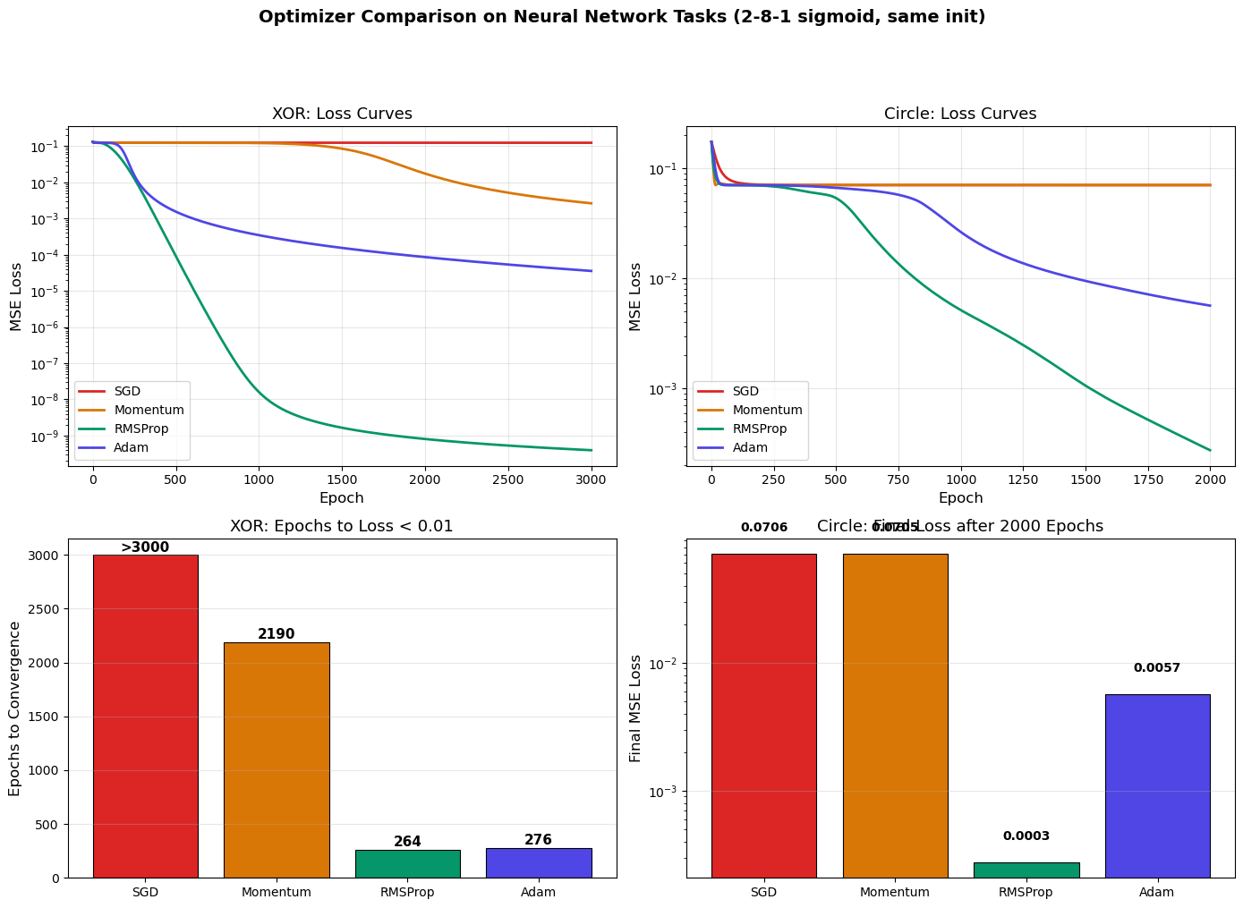
27.5 Optimizer Comparison on Neural Networks#
To demonstrate the practical differences between optimizers, we train the same neural network architecture on two tasks from Chapter 18: XOR classification and circular decision boundaries. We use identical initialization for fair comparison.
First, we define a simplified NeuralNetwork class that supports pluggable optimizers.
# Neural network with pluggable optimizers
# (Simplified from the NeuralNetwork class in Chapter 18)

class NeuralNetwork:
    """Feedforward neural network with backpropagation and pluggable optimizers.

    Implements BP1-BP4 from Chapter 16 with support for SGD, Momentum,
    RMSProp, and Adam optimizers.
    """

    def __init__(self, layer_sizes, activation='sigmoid', rng=None):
        """
        Parameters
        ----------
        layer_sizes : list of int
            Number of neurons in each layer, e.g. [2, 8, 1].
        activation : str
            'sigmoid' or 'relu'.
        rng : np.random.Generator or None
            Random number generator for reproducibility.
        """
        if rng is None:
            rng = np.random.default_rng()
        self.layer_sizes = layer_sizes
        self.L = len(layer_sizes) - 1
        self.activation_name = activation

        # Xavier initialization
        self.weights = []
        self.biases = []
        for l in range(self.L):
            n_in, n_out = layer_sizes[l], layer_sizes[l + 1]
            W = rng.standard_normal((n_out, n_in)) * np.sqrt(2.0 / (n_in + n_out))
            b = np.zeros((n_out, 1))
            self.weights.append(W)
            self.biases.append(b)

        self.z_cache = []
        self.a_cache = []

    def get_params(self):
        """Return flat list of all parameters."""
        params = []
        for l in range(self.L):
            params.append(self.weights[l])
            params.append(self.biases[l])
        return params

    def set_params(self, params):
        """Set parameters from flat list."""
        idx = 0
        for l in range(self.L):
            self.weights[l] = params[idx]
            self.biases[l] = params[idx + 1]
            idx += 2

    def copy_params(self):
        """Return a deep copy of all parameters."""
        return [p.copy() for p in self.get_params()]

    def _activation(self, z):
        if self.activation_name == 'sigmoid':
            return 1.0 / (1.0 + np.exp(-np.clip(z, -500, 500)))
        elif self.activation_name == 'relu':
            return np.maximum(0, z)

    def _activation_derivative(self, z):
        if self.activation_name == 'sigmoid':
            s = self._activation(z)
            return s * (1 - s)
        elif self.activation_name == 'relu':
            return (z > 0).astype(float)

    def forward(self, X):
        """Forward pass. X shape: (n_features, n_samples)."""
        self.z_cache = []
        self.a_cache = [X]
        a = X
        for l in range(self.L):
            z = self.weights[l] @ a + self.biases[l]
            a = self._activation(z)
            self.z_cache.append(z)
            self.a_cache.append(a)
        return a

    def compute_loss(self, y_hat, Y):
        """MSE loss: L = (1/2m) * sum(||y_hat - Y||^2)."""
        m = Y.shape[1]
        return 0.5 * np.sum((y_hat - Y)**2) / m

    def backward(self, Y):
        """Backward pass: compute gradients using BP1-BP4."""
        m = Y.shape[1]
        grads = []  # will hold [dW_0, db_0, dW_1, db_1, ...]

        # Output layer error (BP1)
        a_L = self.a_cache[-1]
        dL_da = (a_L - Y) / m
        sigma_prime = self._activation_derivative(self.z_cache[-1])
        delta = dL_da * sigma_prime

        # Store gradients in order [dW_0, db_0, dW_1, db_1, ...]
        dW_list = [None] * self.L
        db_list = [None] * self.L

        dW_list[-1] = delta @ self.a_cache[-2].T
        db_list[-1] = np.sum(delta, axis=1, keepdims=True)

        # Hidden layers (BP2)
        for l in range(self.L - 2, -1, -1):
            sigma_prime = self._activation_derivative(self.z_cache[l])
            delta = (self.weights[l + 1].T @ delta) * sigma_prime
            dW_list[l] = delta @ self.a_cache[l].T
            db_list[l] = np.sum(delta, axis=1, keepdims=True)

        # Flatten to match get_params() order
        for l in range(self.L):
            grads.append(dW_list[l])
            grads.append(db_list[l])

        return grads

    def train(self, X, Y, epochs, optimizer=None, eta=0.1, verbose=True):
        """Train the network.

        Parameters
        ----------
        X : ndarray, shape (n_features, n_samples)
        Y : ndarray, shape (n_outputs, n_samples)
        epochs : int
        optimizer : object with step(params, grads) method, or None for SGD.
        eta : float
            Learning rate (used only if optimizer is None).
        verbose : bool

        Returns
        -------
        loss_history : list of float
        """
        loss_history = []

        for epoch in range(epochs):
            # Forward
            y_hat = self.forward(X)
            loss = self.compute_loss(y_hat, Y)
            loss_history.append(loss)

            # Backward
            grads = self.backward(Y)

            # Update
            if optimizer is not None:
                params = self.get_params()
                params = optimizer.step(params, grads)
                self.set_params(params)
            else:
                # Vanilla SGD
                params = self.get_params()
                for i in range(len(params)):
                    params[i] = params[i] - eta * grads[i]
                self.set_params(params)

            if verbose and epochs >= 10 and (epoch % (epochs // 10) == 0 or epoch == epochs - 1):
                print(f"Epoch {epoch:5d}/{epochs}: Loss = {loss:.6f}")

        return loss_history


print("NeuralNetwork class defined (with pluggable optimizer support).")
print("Methods: forward, backward, train, get_params, set_params, copy_params")
NeuralNetwork class defined (with pluggable optimizer support).
Methods: forward, backward, train, get_params, set_params, copy_params
Show code cell source
# Optimizer comparison on XOR and Circle tasks

import numpy as np
import matplotlib.pyplot as plt

# --- Data ---
# XOR dataset
X_xor = np.array([[0, 0, 1, 1],
                   [0, 1, 0, 1]], dtype=float)
Y_xor = np.array([[0, 1, 1, 0]], dtype=float)

# Circle dataset
rng_data = np.random.default_rng(42)
n_samples = 300
X_circle = rng_data.uniform(-1, 1, (2, n_samples))
Y_circle = ((X_circle[0]**2 + X_circle[1]**2) < 0.5**2).astype(float).reshape(1, -1)

# --- Shared initialization ---
# Create one network and save its initial parameters
rng_init = np.random.default_rng(123)
nn_ref = NeuralNetwork([2, 8, 1], activation='sigmoid', rng=rng_init)
init_params = nn_ref.copy_params()

# --- Define optimizers ---
optimizer_configs = [
    ('SGD',      None,                                         0.1),
    ('Momentum', MomentumOptimizer(eta=0.1, beta=0.9),         None),
    ('RMSProp',  RMSPropOptimizer(eta=0.01, beta=0.9),         None),
    ('Adam',     AdamOptimizer(eta=0.01, beta1=0.9, beta2=0.999),  None),
]

n_epochs_xor = 3000
n_epochs_circle = 2000

# --- Train on both tasks ---
results = {}  # name -> {'xor_losses': [...], 'circle_losses': [...]}

for name, opt, eta in optimizer_configs:
    results[name] = {}

    # XOR task
    nn = NeuralNetwork([2, 8, 1], activation='sigmoid')
    nn.set_params([p.copy() for p in init_params])
    if opt is not None:
        opt.initialize(nn.get_params()) if hasattr(opt, 'initialize') else None
        if hasattr(opt, 't'):
            opt.t = 0
    losses = nn.train(X_xor, Y_xor, epochs=n_epochs_xor,
                      optimizer=opt, eta=eta if eta else 0.1, verbose=False)
    results[name]['xor_losses'] = losses
    results[name]['xor_final'] = losses[-1]

    # Circle task
    nn2 = NeuralNetwork([2, 8, 1], activation='sigmoid')
    nn2.set_params([p.copy() for p in init_params])
    # Reset optimizer state
    if opt is not None:
        opt.initialize(nn2.get_params()) if hasattr(opt, 'initialize') else None
        if hasattr(opt, 't'):
            opt.t = 0
    losses2 = nn2.train(X_circle, Y_circle, epochs=n_epochs_circle,
                        optimizer=opt, eta=eta if eta else 0.1, verbose=False)
    results[name]['circle_losses'] = losses2
    results[name]['circle_final'] = losses2[-1]

# --- Plot: 4-panel figure ---
fig, axes = plt.subplots(2, 2, figsize=(14, 10))

# XOR loss curves
ax = axes[0, 0]
for name in ['SGD', 'Momentum', 'RMSProp', 'Adam']:
    ax.plot(results[name]['xor_losses'], linewidth=2, color=COLORS[name], label=name)
ax.set_xlabel('Epoch', fontsize=12)
ax.set_ylabel('MSE Loss', fontsize=12)
ax.set_title('XOR: Loss Curves', fontsize=13)
ax.set_yscale('log')
ax.legend(fontsize=10)
ax.grid(True, alpha=0.3)

# Circle loss curves
ax = axes[0, 1]
for name in ['SGD', 'Momentum', 'RMSProp', 'Adam']:
    ax.plot(results[name]['circle_losses'], linewidth=2, color=COLORS[name], label=name)
ax.set_xlabel('Epoch', fontsize=12)
ax.set_ylabel('MSE Loss', fontsize=12)
ax.set_title('Circle: Loss Curves', fontsize=13)
ax.set_yscale('log')
ax.legend(fontsize=10)
ax.grid(True, alpha=0.3)

# XOR: convergence epoch (first epoch where loss < threshold)
ax = axes[1, 0]
threshold = 0.01
bars = []
bar_colors = []
bar_labels = []
for name in ['SGD', 'Momentum', 'RMSProp', 'Adam']:
    losses_arr = results[name]['xor_losses']
    conv_epoch = next((i for i, l in enumerate(losses_arr) if l < threshold), len(losses_arr))
    bars.append(conv_epoch)
    bar_colors.append(COLORS[name])
    bar_labels.append(name)

ax.bar(bar_labels, bars, color=bar_colors, edgecolor='black', linewidth=0.8)
ax.set_ylabel('Epochs to Convergence', fontsize=12)
ax.set_title(f'XOR: Epochs to Loss < {threshold}', fontsize=13)
ax.grid(True, alpha=0.3, axis='y')
for i, v in enumerate(bars):
    label = str(v) if v < n_epochs_xor else f'>{n_epochs_xor}'
    ax.text(i, v + 30, label, ha='center', fontsize=11, fontweight='bold')

# Circle: final loss comparison
ax = axes[1, 1]
final_vals = [results[name]['circle_final'] for name in ['SGD', 'Momentum', 'RMSProp', 'Adam']]
ax.bar(bar_labels, final_vals, color=bar_colors, edgecolor='black', linewidth=0.8)
ax.set_ylabel('Final MSE Loss', fontsize=12)
ax.set_title(f'Circle: Final Loss after {n_epochs_circle} Epochs', fontsize=13)
ax.set_yscale('log')
ax.grid(True, alpha=0.3, axis='y')
for i, v in enumerate(final_vals):
    ax.text(i, v * 1.5, f'{v:.4f}', ha='center', fontsize=10, fontweight='bold')

plt.suptitle('Optimizer Comparison on Neural Network Tasks (2-8-1 sigmoid, same init)',
             fontsize=14, fontweight='bold', y=1.01)
plt.tight_layout(rect=[0, 0, 1, 0.95])
plt.show()

# Print summary table
print("\n" + "=" * 70)
print(f"{'Optimizer':<12} {'XOR Final Loss':>15} {'Circle Final Loss':>18} {'XOR Conv. Epoch':>16}")
print("=" * 70)
for name in ['SGD', 'Momentum', 'RMSProp', 'Adam']:
    xor_loss = results[name]['xor_final']
    circ_loss = results[name]['circle_final']
    losses_arr = results[name]['xor_losses']
    conv = next((i for i, l in enumerate(losses_arr) if l < threshold), n_epochs_xor)
    conv_str = str(conv) if conv < n_epochs_xor else f'>{n_epochs_xor}'
    print(f"{name:<12} {xor_loss:>15.6f} {circ_loss:>18.6f} {conv_str:>16}")
print("=" * 70)
print(f"\nKey insight: Adam (lr=0.01) converges fastest with minimal tuning, while SGD (lr=0.1)")
print(f"requires careful learning rate selection per problem.")
======================================================================
Optimizer     XOR Final Loss  Circle Final Loss  XOR Conv. Epoch
======================================================================
SGD                 0.124916           0.070572            >3000
Momentum            0.002645           0.070500             2190
RMSProp             0.000000           0.000275              264
Adam                0.000036           0.005670              276
======================================================================

Key insight: Adam (lr=0.01) converges fastest with minimal tuning, while SGD (lr=0.1)
requires careful learning rate selection per problem.
27.6 AdamW and Weight Decay#
A subtle but important distinction that went unnoticed for years: L2 regularization and weight decay are NOT the same thing when using adaptive optimizers like Adam.
L2 Regularization vs Weight Decay with SGD#
With vanilla SGD, these two approaches are equivalent:
L2 regularization adds a penalty to the loss:
The gradient becomes:
So the SGD update is:
Weight decay directly shrinks the weights:
Theorem: Equivalence of L2 Regularization and Weight Decay for SGD
For vanilla SGD, L2 regularization with coefficient \(\lambda\) is exactly equivalent to weight decay with coefficient \(\lambda' = \eta\lambda\).
Proof. The SGD update with L2 regularization is:
Setting \(\lambda' = \eta\lambda\), this is identical to the weight decay update \(\mathbf{w}_{t+1} = (1-\lambda')\mathbf{w}_t - \eta \nabla L(\mathbf{w}_t)\). \(\square\)
Why the Equivalence Breaks for Adam#
With Adam, the gradient is scaled by the adaptive factor \(1/\sqrt{\hat{v}_t}\). If we use L2 regularization, the regularization gradient \(\lambda \mathbf{w}_t\) is also scaled by this factor:
where \(\hat{m}_t\) now includes the regularization gradient. This means the weight decay effect is entangled with the adaptive scaling — parameters with large gradients get less regularization, which is not the intended behavior.
Algorithm: AdamW (Loshchilov & Hutter, 2017)
Decoupled weight decay: Apply weight decay directly to the parameters, not through the gradient:
The only change from Adam: the weight decay term \((1-\lambda)\mathbf{w}_t\) is applied outside the adaptive scaling. The gradient used for computing \(\mathbf{m}_t\) and \(\mathbf{v}_t\) is the unregularized gradient \(\nabla L(\mathbf{w}_t)\).
Danger
Many deep learning frameworks implemented “Adam with weight decay” incorrectly for years, using L2 regularization instead of true decoupled weight decay. Loshchilov and Hutter (2017) showed this matters: AdamW consistently outperforms Adam+L2 on tasks like ImageNet classification and language modeling.
Tip
AdamW has become the de facto standard optimizer for training modern deep learning models, including transformers and large language models (LLMs). Nearly every major language model (GPT, BERT, LLaMA, etc.) was trained with AdamW.
Show code cell source
# Demonstrating the difference between L2 regularization and weight decay with Adam
import numpy as np
import matplotlib.pyplot as plt
def run_adam_l2(w_init, eta, lam, beta1=0.9, beta2=0.999, n_steps=200):
"""Adam with L2 regularization (regularization through the gradient)."""
w = w_init.copy()
m = np.zeros_like(w)
v = np.zeros_like(w)
eps = 1e-8
traj = [w.copy()]
for t in range(1, n_steps + 1):
g = grad_quadratic(w) + lam * w # L2: gradient includes regularization
m = beta1 * m + (1 - beta1) * g
v = beta2 * v + (1 - beta2) * g**2
m_hat = m / (1 - beta1**t)
v_hat = v / (1 - beta2**t)
w = w - eta * m_hat / (np.sqrt(v_hat) + eps)
traj.append(w.copy())
return np.array(traj)
def run_adamw(w_init, eta, lam, beta1=0.9, beta2=0.999, n_steps=200):
"""AdamW: decoupled weight decay."""
w = w_init.copy()
m = np.zeros_like(w)
v = np.zeros_like(w)
eps = 1e-8
traj = [w.copy()]
for t in range(1, n_steps + 1):
g = grad_quadratic(w) # Unregularized gradient
m = beta1 * m + (1 - beta1) * g
v = beta2 * v + (1 - beta2) * g**2
m_hat = m / (1 - beta1**t)
v_hat = v / (1 - beta2**t)
w = (1 - lam) * w - eta * m_hat / (np.sqrt(v_hat) + eps) # Decoupled decay
traj.append(w.copy())
return np.array(traj)
w_init = np.array([5.0, 0.5])
eta = 0.1
lam = 0.01
n_steps = 200
traj_l2 = run_adam_l2(w_init, eta, lam, n_steps=n_steps)
traj_w = run_adamw(w_init, eta, lam, n_steps=n_steps)
fig, axes = plt.subplots(1, 2, figsize=(14, 5))
# Trajectories
ax = axes[0]
w1_grid = np.linspace(-6, 6, 300)
w2_grid = np.linspace(-1.0, 1.0, 300)
W1, W2 = np.meshgrid(w1_grid, w2_grid)
Z = W1**2 + 50.0 * W2**2
levels = [0.5, 1, 2, 5, 10, 15, 20, 30, 50]
ax.contour(W1, W2, Z, levels=levels, colors='gray', alpha=0.5, linewidths=0.8)
ax.contourf(W1, W2, Z, levels=levels, cmap='Blues', alpha=0.12)
ax.plot(traj_l2[:, 0], traj_l2[:, 1], 'o-', color='#e11d48', markersize=2,
linewidth=0.8, label='Adam + L2')
ax.plot(traj_w[:, 0], traj_w[:, 1], 'o-', color=COLORS['Adam'], markersize=2,
linewidth=0.8, label='AdamW')
ax.plot(0, 0, '*', color='gold', markersize=14, markeredgecolor='black',
markeredgewidth=1, zorder=6)
ax.set_xlabel('$w_1$', fontsize=12)
ax.set_ylabel('$w_2$', fontsize=12)
ax.set_title('Adam+L2 vs AdamW Trajectories', fontsize=13)
ax.set_xlim(-6, 6)
ax.set_ylim(-1.0, 1.0)
ax.legend(fontsize=11)
ax.grid(True, alpha=0.2)
# Loss curves
ax = axes[1]
losses_l2 = [ill_conditioned_quadratic(w) for w in traj_l2]
losses_w = [ill_conditioned_quadratic(w) for w in traj_w]
ax.plot(losses_l2, linewidth=2, color='#e11d48', label='Adam + L2')
ax.plot(losses_w, linewidth=2, color=COLORS['Adam'], label='AdamW')
ax.set_xlabel('Step', fontsize=12)
ax.set_ylabel('Loss (unregularized)', fontsize=12)
ax.set_title('Loss Curves: Adam+L2 vs AdamW', fontsize=13)
ax.set_yscale('log')
ax.legend(fontsize=11)
ax.grid(True, alpha=0.3)
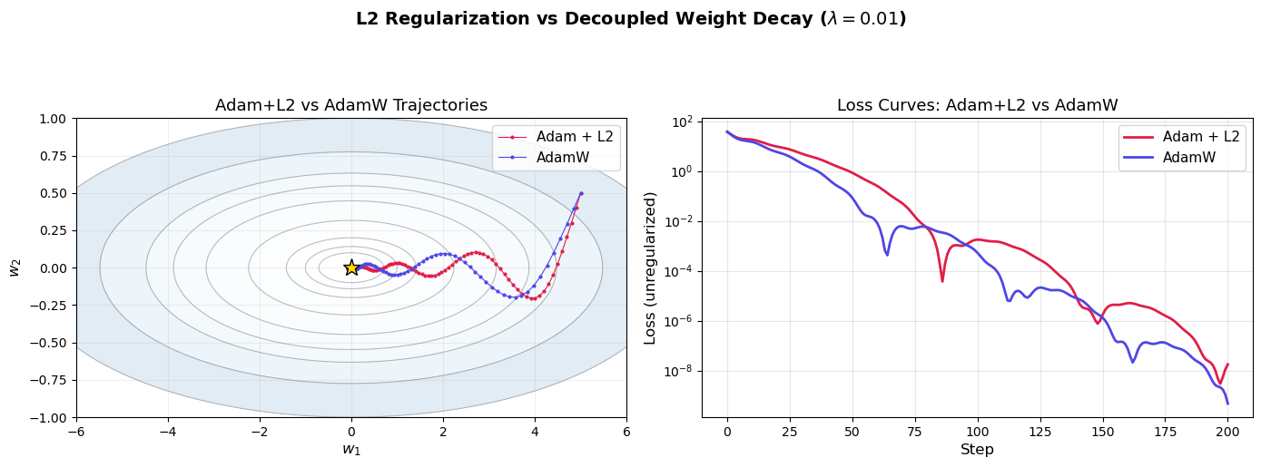
plt.suptitle(f'L2 Regularization vs Decoupled Weight Decay ($\\lambda = {lam}$)',
fontsize=14, fontweight='bold', y=1.02)
plt.tight_layout(rect=[0, 0, 1, 0.93])
plt.show()
print(f"Final losses after {n_steps} steps:")
print(f" Adam + L2: {ill_conditioned_quadratic(traj_l2[-1]):.6f}")
print(f" AdamW: {ill_conditioned_quadratic(traj_w[-1]):.6f}")
print(f"\nThe trajectories differ because L2 regularization passes through Adam's")
print(f"adaptive scaling, while AdamW applies weight decay directly.")
Final losses after 200 steps:
  Adam + L2:  0.000000
  AdamW:      0.000000

The trajectories differ because L2 regularization passes through Adam's
adaptive scaling, while AdamW applies weight decay directly.
Exercises#
Exercise 27.1. Implement the Nesterov Accelerated Gradient optimizer as a class
(similar to MomentumOptimizer but with the lookahead gradient evaluation). Test it on
the ill-conditioned quadratic \(L = w_1^2 + 50\,w_2^2\) and compare convergence with
standard momentum. Then apply it to the XOR task using the NeuralNetwork class.
Exercise 27.2. Prove the momentum convergence bound for quadratic objectives. Consider \(L(\mathbf{w}) = \frac{1}{2}\mathbf{w}^T \mathbf{A}\mathbf{w}\) where \(\mathbf{A} = \mathrm{diag}(\lambda_1, \lambda_2)\) with \(\lambda_1 = 1\) and \(\lambda_2 = \kappa\). Write the momentum update as a linear recurrence \(\begin{pmatrix} w_{t+1} \\ w_t \end{pmatrix} = \mathbf{M} \begin{pmatrix} w_t \\ w_{t-1}\end{pmatrix}\) and show that the spectral radius of \(\mathbf{M}\) with optimal \(\eta\) and \(\beta\) is \(\frac{\sqrt{\kappa}-1}{\sqrt{\kappa}+1}\).
Exercise 27.3. Investigate the effect of Adam’s bias correction empirically. Implement Adam without bias correction (i.e., use \(\mathbf{m}_t\) and \(\mathbf{v}_t\) directly instead of \(\hat{\mathbf{m}}_t\) and \(\hat{\mathbf{v}}_t\)). Train the 2-8-1 network on the circle dataset with both versions and compare the first 100 epochs. How much does bias correction matter?
Exercise 27.4. Create a learning rate sensitivity experiment. For each optimizer (SGD, Momentum, RMSProp, Adam), train on XOR with learning rates \(\eta \in \{0.0001, 0.001, 0.01, 0.1, 1.0\}\) and plot final loss vs learning rate. Which optimizer is most robust to the choice of learning rate?
Exercise 27.5. Implement the AdamW optimizer as a class (extend the AdamOptimizer
with a weight_decay parameter). Apply it to the function approximation task from
Chapter 18 (\(\sin(x)\) with a 1-16-1 network) and compare with standard Adam.
Exercise 27.6. (Challenging) Implement learning rate warmup for Adam: start with \(\eta = 0\) and linearly increase to the target \(\eta\) over the first \(T_{\text{warmup}}\) epochs, then hold constant. Test with \(T_{\text{warmup}} \in \{0, 50, 100, 200\}\) on the circle classification task. Does warmup help? Why might it be important for training large models?