Chapter 11: Breaking Through — Multi-Layer Networks#
The Power of Composition#
The previous chapters established the severe limitations of single-layer perceptrons: they cannot compute XOR, parity, connectedness, or any non-linearly-separable function. The natural question is: can these limitations be overcome by adding more layers?
The answer is a resounding yes. In this chapter, we show that a network with just one hidden layer can solve XOR, compute parity of any number of bits, and — as we will preview — approximate any continuous function to arbitrary accuracy.
The key insight is deceptively simple: hidden layers learn new representations. The hidden neurons transform the input into a new coordinate system where the previously inseparable classes become separable. This idea — that the right representation makes hard problems easy — is the fundamental principle underlying all of deep learning.
Danger
Even though multi-layer networks CAN solve XOR, in 1969 there was no broadly effective training algorithm for multi-layer networks. The solution existed but nobody knew how to find it automatically!
This distinction was central to the period’s skepticism about neural networks. The XOR-solving network we construct in this chapter uses hand-designed weights. In 1969, if you knew the target function (like XOR), you could manually design a network to compute it. But in real applications, you do NOT know the target function — you only have training examples. Without a learning algorithm that could automatically adjust the weights of hidden layers, multi-layer networks were a theoretical curiosity, not a practical tool.
The backpropagation algorithm, which solves this problem, was described by Werbos in 1974 and popularized by Rumelhart, Hinton, and Williams in 1986.
Tip
Hidden layer = learned feature transformation (the key insight of deep learning).
The hidden layer does not just add more parameters — it performs a nonlinear coordinate transformation. It maps the input into a new “feature space” where the problem becomes linearly separable. This is the same idea behind kernel methods, but with a crucial difference: in a neural network, the transformation is learned from data rather than chosen by the practitioner.
In modern deep learning, networks with many hidden layers learn hierarchies of increasingly abstract features:
Image recognition: edges -> textures -> parts -> objects
Language: characters -> words -> phrases -> meaning
Speech: waveforms -> phonemes -> words -> sentences
It all starts here, with two hidden neurons solving XOR.
Note
The gap: 1969–1986 — 17 years until backpropagation made multi-layer networks trainable.
The timeline of this gap is remarkable:
1969: Minsky and Papert prove single-layer limitations. Multi-layer solutions exist but cannot be found automatically.
1974: Paul Werbos describes backpropagation in his PhD thesis at Harvard. Almost nobody notices.
1982: John Hopfield revives interest in neural networks with his associative memory model.
1985: David Parker independently rediscovers backpropagation.
1986: Rumelhart, Hinton, and Williams publish backpropagation in Nature. The neural network renaissance begins.
During these 17 years, the solution to the credit assignment problem (how to train hidden layers) existed but was buried in an obscure thesis. Meanwhile, the AI community was focused on expert systems and symbolic AI. The delay was historically significant.
Show code cell source
import numpy as np
import matplotlib.pyplot as plt
from matplotlib.patches import FancyArrowPatch

plt.rcParams.update({
    'figure.figsize': (8, 6),
    'font.size': 12,
    'axes.grid': True,
    'grid.alpha': 0.3
})

def step(z):
    """Heaviside step function."""
    return (np.array(z) >= 0).astype(int)
1. XOR: Two Constructions#
We present two different 2-layer network architectures for computing XOR, each with a distinct geometric interpretation.
Theorem (XOR with Two Hidden Neurons)
The XOR function can be computed by a neural network with 2 input neurons, 2 hidden neurons (with step activation), and 1 output neuron (with step activation). Two distinct constructions achieve this:
Construction 1 (OR + NAND + AND):
Hidden neuron 1 (OR): \(h_1 = \text{step}(x_1 + x_2 - 0.5)\)
Hidden neuron 2 (NAND): \(h_2 = \text{step}(-x_1 - x_2 + 1.5)\)
Output neuron (AND): \(y = \text{step}(h_1 + h_2 - 1.5)\)
Construction 2 (Dual Threshold / Band):
Hidden neuron 1: \(h_1 = \text{step}(x_1 + x_2 - 0.5)\) (fires when sum \(\geq 1\))
Hidden neuron 2: \(h_2 = \text{step}(x_1 + x_2 - 1.5)\) (fires when sum \(\geq 2\))
Output neuron: \(y = \text{step}(h_1 - h_2 - 0.5)\) (fires when \(h_1=1, h_2=0\))
Moreover, 2 hidden neurons are necessary — 1 hidden neuron is provably insufficient.
Show code cell source
# Full verification of both XOR constructions

X = np.array([[0, 0], [0, 1], [1, 0], [1, 1]])
y_true = np.array([0, 1, 1, 0])

print("=" * 70)
print("CONSTRUCTION 1: OR + NAND + AND")
print("=" * 70)
print(f"{'x1':>3} {'x2':>3} | {'h1=OR':>7} {'h2=NAND':>8} | {'y=AND':>6} {'target':>7} {'status':>7}")
print("-" * 70)

all_correct_1 = True
for i in range(4):
    x1, x2 = X[i]
    h1 = step(x1 + x2 - 0.5)
    h2 = step(-x1 - x2 + 1.5)
    y_pred = step(h1 + h2 - 1.5)
    ok = 'OK' if y_pred == y_true[i] else 'FAIL'
    if y_pred != y_true[i]: all_correct_1 = False
    print(f"{x1:>3.0f} {x2:>3.0f} | {h1:>7} {h2:>8} | {y_pred:>6} {y_true[i]:>7} {ok:>7}")

print(f"\nResult: {'ALL CORRECT' if all_correct_1 else 'ERRORS FOUND'}")

print()
print("=" * 70)
print("CONSTRUCTION 2: Dual Threshold (Band)")
print("=" * 70)
print(f"{'x1':>3} {'x2':>3} | {'sum':>4} {'h1(>=1)':>8} {'h2(>=2)':>8} | {'y':>3} {'target':>7} {'status':>7}")
print("-" * 70)

all_correct_2 = True
for i in range(4):
    x1, x2 = X[i]
    s = x1 + x2
    h1 = step(s - 0.5)
    h2 = step(s - 1.5)
    y_pred = step(h1 - h2 - 0.5)
    ok = 'OK' if y_pred == y_true[i] else 'FAIL'
    if y_pred != y_true[i]: all_correct_2 = False
    print(f"{x1:>3.0f} {x2:>3.0f} | {s:>4.0f} {h1:>8} {h2:>8} | {y_pred:>3} {y_true[i]:>7} {ok:>7}")

print(f"\nResult: {'ALL CORRECT' if all_correct_2 else 'ERRORS FOUND'}")
======================================================================
CONSTRUCTION 1: OR + NAND + AND
======================================================================
 x1  x2 |   h1=OR  h2=NAND |  y=AND  target  status
----------------------------------------------------------------------
  0   0 |       0        1 |      0       0      OK
  0   1 |       1        1 |      1       1      OK
  1   0 |       1        1 |      1       1      OK
  1   1 |       1        0 |      0       0      OK

Result: ALL CORRECT

======================================================================
CONSTRUCTION 2: Dual Threshold (Band)
======================================================================
 x1  x2 |  sum  h1(>=1)  h2(>=2) |   y  target  status
----------------------------------------------------------------------
  0   0 |    0        0        0 |   0       0      OK
  0   1 |    1        1        0 |   1       1      OK
  1   0 |    1        1        0 |   1       1      OK
  1   1 |    2        1        1 |   0       0      OK

Result: ALL CORRECT
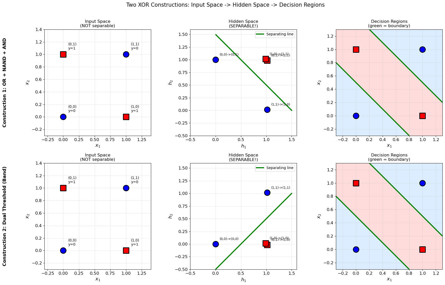
2. Geometric Interpretation#
The hidden layer performs a nonlinear coordinate transformation from the original input space to a new “hidden space” where the classes become linearly separable.
For Construction 1 (OR + NAND), the mapping is:
\((x_1, x_2)\) |
\((h_1, h_2)\) |
XOR |
|---|---|---|
\((0, 0)\) |
\((0, 1)\) |
0 |
\((0, 1)\) |
\((1, 1)\) |
1 |
\((1, 0)\) |
\((1, 1)\) |
1 |
\((1, 1)\) |
\((1, 0)\) |
0 |
For Construction 2 (Band), the mapping is:
\((x_1, x_2)\) |
\((h_1, h_2)\) |
XOR |
|---|---|---|
\((0, 0)\) |
\((0, 0)\) |
0 |
\((0, 1)\) |
\((1, 0)\) |
1 |
\((1, 0)\) |
\((1, 0)\) |
1 |
\((1, 1)\) |
\((1, 1)\) |
0 |
In both cases, the hidden representation collapses the two XOR=1 points onto a single point, making separation trivial.

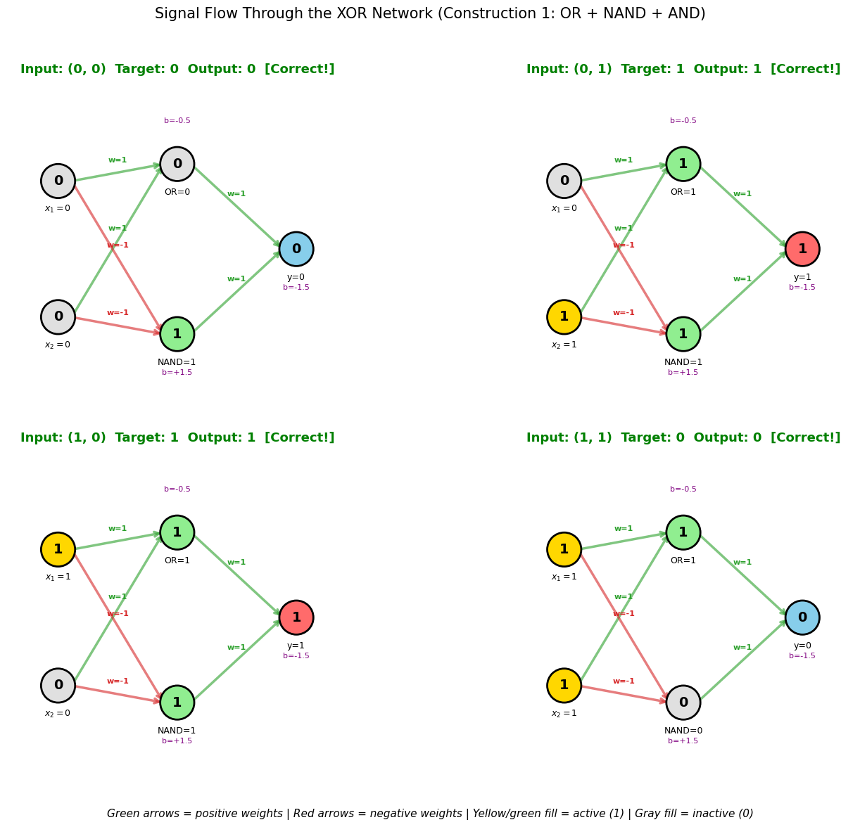
2b. Interactive Network Diagram: Signal Flow Through the XOR Network#
The following diagram traces the signal flow for each of the 4 XOR inputs through the network, showing the activation at each neuron.
Show code cell source
import numpy as np
import matplotlib.pyplot as plt
import matplotlib.patches as mpatches

def step(z):
    return (np.array(z) >= 0).astype(int)

X = np.array([[0, 0], [0, 1], [1, 0], [1, 1]])
y_true = np.array([0, 1, 1, 0])

fig, axes = plt.subplots(2, 2, figsize=(16, 12))

for idx in range(4):
    ax = axes[idx // 2][idx % 2]
    x1, x2 = X[idx]

    # Compute activations
    h1 = int(x1 + x2 - 0.5 >= 0)   # OR
    h2 = int(-x1 - x2 + 1.5 >= 0)  # NAND
    y_out = int(h1 + h2 - 1.5 >= 0) # AND

    # Neuron positions
    positions = {
        'x1': (0.1, 0.7), 'x2': (0.1, 0.3),
        'h1': (0.45, 0.75), 'h2': (0.45, 0.25),
        'y': (0.8, 0.5)
    }

    # Draw connections with weights
    connections = [
        ('x1', 'h1', 1.0), ('x2', 'h1', 1.0),     # to OR
        ('x1', 'h2', -1.0), ('x2', 'h2', -1.0),   # to NAND
        ('h1', 'y', 1.0), ('h2', 'y', 1.0),        # to AND
    ]

    for src, dst, w in connections:
        x_s, y_s = positions[src]
        x_d, y_d = positions[dst]
        color = '#2ca02c' if w > 0 else '#d62728'
        lw = abs(w) * 2.5
        ax.annotate('', xy=(x_d - 0.04, y_d), xytext=(x_s + 0.04, y_s),
                    arrowprops=dict(arrowstyle='->', color=color,
                                   linewidth=lw, alpha=0.6))
        # Weight label
        mx, my = (x_s + x_d) / 2, (y_s + y_d) / 2
        ax.text(mx, my + 0.03, f'w={w:.0f}', fontsize=8, ha='center',
                color=color, fontweight='bold')

    # Draw neurons
    neuron_data = {
        'x1': (x1, f'$x_1={x1:.0f}$'),
        'x2': (x2, f'$x_2={x2:.0f}$'),
        'h1': (h1, f'OR={h1}'),
        'h2': (h2, f'NAND={h2}'),
        'y': (y_out, f'y={y_out}')
    }

    for name, (val, label) in neuron_data.items():
        x_n, y_n = positions[name]
        # Color based on activation
        if name in ['x1', 'x2']:
            fcolor = '#FFD700' if val == 1 else '#E0E0E0'
        elif name == 'y':
            fcolor = '#FF6B6B' if val == 1 else '#87CEEB'
        else:
            fcolor = '#90EE90' if val == 1 else '#E0E0E0'

        circle = plt.Circle((x_n, y_n), 0.05, facecolor=fcolor,
                           edgecolor='black', linewidth=2, zorder=10)
        ax.add_patch(circle)
        ax.text(x_n, y_n, str(int(val)), ha='center', va='center',
                fontsize=14, fontweight='bold', zorder=11)
        ax.text(x_n, y_n - 0.09, label, ha='center', fontsize=9, zorder=11)

    # Bias labels
    ax.text(0.45, 0.87, 'b=-0.5', fontsize=8, ha='center', color='purple')
    ax.text(0.45, 0.13, 'b=+1.5', fontsize=8, ha='center', color='purple')
    ax.text(0.8, 0.38, 'b=-1.5', fontsize=8, ha='center', color='purple')

    # Title
    correct = 'Correct!' if y_out == y_true[idx] else 'WRONG!'
    color_t = 'green' if y_out == y_true[idx] else 'red'
    ax.set_title(f'Input: ({x1:.0f}, {x2:.0f})  Target: {y_true[idx]}  '
                 f'Output: {y_out}  [{correct}]',
                 fontsize=13, fontweight='bold', color=color_t)

    ax.set_xlim(-0.05, 0.95)
    ax.set_ylim(0.0, 1.0)
    ax.set_aspect('equal')
    ax.axis('off')

# Legend
fig.text(0.5, 0.02,
         'Green arrows = positive weights | Red arrows = negative weights | '
         'Yellow/green fill = active (1) | Gray fill = inactive (0)',
         ha='center', fontsize=11, style='italic')

plt.suptitle('Signal Flow Through the XOR Network (Construction 1: OR + NAND + AND)',
             fontsize=15, y=0.98)
plt.tight_layout(rect=[0, 0.04, 1, 0.96])
plt.show()
3. The Feature Space Idea#
The two-layer XOR network illustrates what is arguably the fundamental idea of deep learning:
Hidden layers learn representations. The hidden neurons transform the input into a new coordinate system (the “feature space” or “representation space”) where the task becomes easy.
Why This Matters#
In the XOR example:
Input space \((x_1, x_2)\): the task is impossible for a linear classifier.
Hidden space \((h_1, h_2)\): the task becomes trivially easy.
The hidden layer has performed a nonlinear feature extraction that makes the problem linearly separable. This is exactly what happens in deep neural networks, but at a much larger scale:
In image recognition, early layers detect edges, middle layers detect textures and parts, and late layers detect objects.
In language models, layers progressively transform raw text into semantic representations.
Connection to the Kernel Trick#
The idea of mapping data to a higher-dimensional feature space where it becomes linearly separable is also the foundation of kernel methods (Chapter 10). The key difference:
Kernel methods: the feature map \(\varphi\) is fixed (chosen by the practitioner).
Neural networks: the feature map is learned from data (via the hidden layer weights).
Learning the representation is both the great strength and the great challenge of neural networks.
4. Building Larger Networks#
To explore multi-layer networks systematically, we implement a general-purpose MultiLayerNetwork class with step activation and configurable architecture.
class MultiLayerNetwork:
    """A multi-layer network with step activation.

    Forward pass only (no learning). Weights are set manually.

    Parameters
    ----------
    layer_sizes : list of int
        Number of neurons in each layer, including input.
        Example: [2, 2, 1] means 2 inputs, 2 hidden, 1 output.
    """

    def __init__(self, layer_sizes):
        self.layer_sizes = layer_sizes
        self.n_layers = len(layer_sizes) - 1  # number of weight layers

        # Initialize weights and biases to zeros
        self.weights = []
        self.biases = []
        for i in range(self.n_layers):
            W = np.zeros((layer_sizes[i+1], layer_sizes[i]))
            b = np.zeros(layer_sizes[i+1])
            self.weights.append(W)
            self.biases.append(b)

    def set_weights(self, layer_idx, W, b):
        """Set weights and biases for a specific layer.

        Parameters
        ----------
        layer_idx : int
            Index of the layer (0 = first weight layer).
        W : array of shape (n_out, n_in)
            Weight matrix.
        b : array of shape (n_out,)
            Bias vector.
        """
        self.weights[layer_idx] = np.array(W, dtype=float)
        self.biases[layer_idx] = np.array(b, dtype=float)

    def forward(self, x):
        """Forward pass through the network.

        Parameters
        ----------
        x : array of shape (n_input,)
            Input vector.

        Returns
        -------
        output : array
            Network output.
        activations : list of arrays
            Activations at each layer (including input).
        """
        activations = [np.array(x, dtype=float)]
        a = activations[0]

        for i in range(self.n_layers):
            z = self.weights[i] @ a + self.biases[i]
            a = step(z)
            activations.append(a)

        return a, activations

    def predict(self, x):
        """Return just the output (no intermediate activations)."""
        output, _ = self.forward(x)
        return output

    def summary(self):
        """Print network architecture summary."""
        print(f"Network: {' -> '.join(str(s) for s in self.layer_sizes)}")
        total_params = 0
        for i in range(self.n_layers):
            n_params = self.weights[i].size + self.biases[i].size
            total_params += n_params
            print(f"  Layer {i}: {self.layer_sizes[i]} -> {self.layer_sizes[i+1]} "
                  f"({self.weights[i].shape[1]}x{self.weights[i].shape[0]} weights + "
                  f"{self.biases[i].size} biases = {n_params} params)")
        print(f"  Total parameters: {total_params}")


# Test with XOR (Construction 1)
net = MultiLayerNetwork([2, 2, 1])
net.set_weights(0,
    W=[[1, 1], [-1, -1]],     # hidden layer: OR, NAND
    b=[-0.5, 1.5])            # biases
net.set_weights(1,
    W=[[1, 1]],               # output layer: AND
    b=[-1.5])                 # bias

net.summary()
print()

print("XOR verification:")
for i in range(4):
    output, acts = net.forward(X[i])
    print(f"  Input {X[i]} -> Hidden {acts[1]} -> Output {output[0]:.0f} (target: {y_true[i]})")
Network: 2 -> 2 -> 1
  Layer 0: 2 -> 2 (2x2 weights + 2 biases = 6 params)
  Layer 1: 2 -> 1 (2x1 weights + 1 biases = 3 params)
  Total parameters: 9

XOR verification:
  Input [0 0] -> Hidden [0 1] -> Output 0 (target: 0)
  Input [0 1] -> Hidden [1 1] -> Output 1 (target: 1)
  Input [1 0] -> Hidden [1 1] -> Output 1 (target: 1)
  Input [1 1] -> Hidden [1 0] -> Output 0 (target: 0)
5. 3-Bit Parity#
The 3-bit parity function outputs 1 when an odd number of inputs are 1:
Truth Table#
\(x_1\) |
\(x_2\) |
\(x_3\) |
Parity |
|---|---|---|---|
0 |
0 |
0 |
0 |
0 |
0 |
1 |
1 |
0 |
1 |
0 |
1 |
0 |
1 |
1 |
0 |
1 |
0 |
0 |
1 |
1 |
0 |
1 |
0 |
1 |
1 |
0 |
0 |
1 |
1 |
1 |
1 |
Decomposition#
We can compute 3-bit parity as:
This requires cascading two XOR computations. Each XOR needs 2 hidden neurons, but we can organize this into layers.
Show code cell source
# 3-bit parity: decomposition into cascaded XOR operations

X3 = np.array([[0,0,0], [0,0,1], [0,1,0], [0,1,1],
               [1,0,0], [1,0,1], [1,1,0], [1,1,1]])
y3 = np.array([0, 1, 1, 0, 1, 0, 0, 1])

# Architecture: 3 inputs -> 2 hidden (layer 1) -> 2 hidden (layer 2) -> 1 output
# Layer 1: compute XOR(x1, x2) using OR + NAND
#   h1_1 = step(x1 + x2 - 0.5)           [OR(x1,x2)]
#   h1_2 = step(-x1 - x2 + 1.5)          [NAND(x1,x2)]
# Then XOR(x1,x2) = AND(h1_1, h1_2) = step(h1_1 + h1_2 - 1.5)
#
# Layer 2: compute XOR(XOR(x1,x2), x3) using similar logic
# But we need to feed both h1_1, h1_2, and x3 to this layer.
#
# Alternative: Use a 3-layer network: 3 -> 2 -> 3 -> 1
# Or use a direct approach with 4 hidden neurons in one layer.

# Direct single-hidden-layer approach:
# XOR(x1,x2,x3) = 1 iff exactly 1 or 3 inputs are 1
# i.e., sum in {1, 3}
#
# We can use 3 "band" neurons:
# h1 = step(x1+x2+x3 - 0.5)   fires when sum >= 1
# h2 = step(x1+x2+x3 - 1.5)   fires when sum >= 2
# h3 = step(x1+x2+x3 - 2.5)   fires when sum >= 3
#
# Parity = h1 - h2 + h3 (evaluate: sum=0: 0, sum=1: 1, sum=2: 0, sum=3: 1)
# But h1-h2+h3 can be 0 or 1, so y = step(h1 - h2 + h3 - 0.5)

print("3-Bit Parity: Single Hidden Layer with 3 Neurons")
print("="*60)

net3 = MultiLayerNetwork([3, 3, 1])
net3.set_weights(0,
    W=[[1, 1, 1],      # h1: fires when sum >= 1
       [1, 1, 1],      # h2: fires when sum >= 2
       [1, 1, 1]],     # h3: fires when sum >= 3
    b=[-0.5, -1.5, -2.5])

net3.set_weights(1,
    W=[[1, -1, 1]],    # y = step(h1 - h2 + h3 - 0.5)
    b=[-0.5])

net3.summary()
print()

print(f"{'x1':>3} {'x2':>3} {'x3':>3} | {'sum':>4} {'h1':>4} {'h2':>4} {'h3':>4} | {'y':>3} {'target':>7} {'ok':>4}")
print("-" * 60)

all_correct = True
for i in range(8):
    output, acts = net3.forward(X3[i])
    h = acts[1]
    s = sum(X3[i])
    ok = 'OK' if output[0] == y3[i] else 'FAIL'
    if output[0] != y3[i]: all_correct = False
    print(f"{X3[i][0]:>3.0f} {X3[i][1]:>3.0f} {X3[i][2]:>3.0f} | {s:>4.0f} {h[0]:>4.0f} {h[1]:>4.0f} {h[2]:>4.0f} | {output[0]:>3.0f} {y3[i]:>7} {ok:>4}")

print(f"\nResult: {'ALL CORRECT' if all_correct else 'ERRORS FOUND'}")
print("\nNote: Only 3 hidden neurons needed for 3-bit parity!")
print("The trick: h1,h2,h3 encode the sum, and the output checks if sum is odd.")
3-Bit Parity: Single Hidden Layer with 3 Neurons
============================================================
Network: 3 -> 3 -> 1
  Layer 0: 3 -> 3 (3x3 weights + 3 biases = 12 params)
  Layer 1: 3 -> 1 (3x1 weights + 1 biases = 4 params)
  Total parameters: 16

 x1  x2  x3 |  sum   h1   h2   h3 |   y  target   ok
------------------------------------------------------------
  0   0   0 |    0    0    0    0 |   0       0   OK
  0   0   1 |    1    1    0    0 |   1       1   OK
  0   1   0 |    1    1    0    0 |   1       1   OK
  0   1   1 |    2    1    1    0 |   0       0   OK
  1   0   0 |    1    1    0    0 |   1       1   OK
  1   0   1 |    2    1    1    0 |   0       0   OK
  1   1   0 |    2    1    1    0 |   0       0   OK
  1   1   1 |    3    1    1    1 |   1       1   OK

Result: ALL CORRECT

Note: Only 3 hidden neurons needed for 3-bit parity!
The trick: h1,h2,h3 encode the sum, and the output checks if sum is odd.
Show code cell source
# Alternative: Cascaded XOR approach (2 layers of hidden neurons)

print("3-Bit Parity: Cascaded XOR (2 Hidden Layers)")
print("="*60)
print("Architecture: 3 -> 2 -> 2 -> 1")
print("  Layer 1: Compute OR(x1,x2) and NAND(x1,x2)")
print("  Layer 2: Combine to get XOR(x1,x2), then start XOR with x3")
print()

# This requires carrying x3 through, so we need a slightly different architecture.
# Let's use: 3 -> 3 -> 2 -> 1
# Layer 1: h1=OR(x1,x2), h2=NAND(x1,x2), h3=x3 (passthrough)
# Layer 2: compute XOR of (AND(h1,h2), h3)
#   = OR(AND(h1,h2), h3) AND NAND(AND(h1,h2), h3)
# But AND(h1,h2) is not directly available...

# Simpler: 3 -> 4 -> 1
# Directly compute with 4 hidden neurons
# h1 = step(x1+x2+x3-0.5)   [at least 1]
# h2 = step(x1+x2+x3-1.5)   [at least 2]
# h3 = step(x1+x2+x3-2.5)   [at least 3]
# h4 = ... (not needed, 3 suffice as shown above)

# Instead, let's demonstrate the cascaded approach with manual computation
def parity3_cascaded(x):
    """Compute 3-bit parity via cascaded XOR."""
    x1, x2, x3 = x

    # Stage 1: XOR(x1, x2)
    a1 = step(x1 + x2 - 0.5)      # OR(x1, x2)
    a2 = step(-x1 - x2 + 1.5)     # NAND(x1, x2)
    xor12 = step(a1 + a2 - 1.5)   # AND(OR, NAND) = XOR

    # Stage 2: XOR(xor12, x3)
    b1 = step(xor12 + x3 - 0.5)   # OR(xor12, x3)
    b2 = step(-xor12 - x3 + 1.5)  # NAND(xor12, x3)
    result = step(b1 + b2 - 1.5)  # AND(OR, NAND) = XOR

    return result, (a1, a2, xor12, b1, b2)

print("Cascaded XOR computation:")
print(f"{'x1 x2 x3':>8} | {'OR12':>5} {'NAND12':>7} {'XOR12':>6} | {'OR_3':>5} {'NAND_3':>7} | {'result':>7} {'target':>7}")
print("-" * 75)

for i in range(8):
    result, intermediates = parity3_cascaded(X3[i])
    a1, a2, xor12, b1, b2 = intermediates
    ok = 'OK' if result == y3[i] else 'FAIL'
    print(f"{X3[i][0]:.0f}  {X3[i][1]:.0f}  {X3[i][2]:.0f}  | {a1:>5.0f} {a2:>7.0f} {xor12:>6.0f} | "
          f"{b1:>5.0f} {b2:>7.0f} | {result:>7.0f} {y3[i]:>7}  {ok}")

print("\nCascaded approach: 4 hidden neurons across 2 layers (+ 1 output).")
print("Direct approach: 3 hidden neurons in 1 layer (+ 1 output).")
print("The direct approach is more efficient for this problem!")
3-Bit Parity: Cascaded XOR (2 Hidden Layers)
============================================================
Architecture: 3 -> 2 -> 2 -> 1
  Layer 1: Compute OR(x1,x2) and NAND(x1,x2)
  Layer 2: Combine to get XOR(x1,x2), then start XOR with x3

Cascaded XOR computation:
x1 x2 x3 |  OR12  NAND12  XOR12 |  OR_3  NAND_3 |  result  target
---------------------------------------------------------------------------
0  0  0  |     0       1      0 |     0       1 |       0       0  OK
0  0  1  |     0       1      0 |     1       1 |       1       1  OK
0  1  0  |     1       1      1 |     1       1 |       1       1  OK
0  1  1  |     1       1      1 |     1       0 |       0       0  OK
1  0  0  |     1       1      1 |     1       1 |       1       1  OK
1  0  1  |     1       1      1 |     1       0 |       0       0  OK
1  1  0  |     1       0      0 |     0       1 |       0       0  OK
1  1  1  |     1       0      0 |     1       1 |       1       1  OK

Cascaded approach: 4 hidden neurons across 2 layers (+ 1 output).
Direct approach: 3 hidden neurons in 1 layer (+ 1 output).
The direct approach is more efficient for this problem!
6. n-Bit Parity#
The constructions above generalize to \(n\)-bit parity.
Contrast with Minsky-Papert#
Minsky and Papert proved that a single-layer perceptron needs order \(n\) to compute parity — meaning it must examine all \(n\) inputs simultaneously in at least one partial predicate. A multi-layer network, by contrast, needs only \(O(n)\) neurons. The limitation is in the single-layer architecture, not in neural networks per se.
Show code cell source
# n-bit parity: general implementation and verification

def build_parity_network(n):
    """Build a network computing n-bit parity using the direct construction."""
    net = MultiLayerNetwork([n, n, 1])

    # Hidden layer: h_k fires when sum >= k
    W_hidden = np.ones((n, n))  # all weights = 1
    b_hidden = np.array([-(k + 0.5) for k in range(n)])  # thresholds at k+0.5
    net.set_weights(0, W_hidden, b_hidden)

    # Output layer: alternating signs
    W_output = np.array([[(-1)**(k) for k in range(n)]])  # +1, -1, +1, ...
    b_output = np.array([-0.5])
    net.set_weights(1, W_output, b_output)

    return net


# Test for n = 2, 3, 4, 5
for n in [2, 3, 4, 5]:
    net = build_parity_network(n)

    # Generate all 2^n inputs
    all_inputs = np.array([[int(b) for b in format(i, f'0{n}b')] for i in range(2**n)])
    true_parity = np.sum(all_inputs, axis=1) % 2

    # Test
    correct = 0
    for i in range(len(all_inputs)):
        pred = net.predict(all_inputs[i])[0]
        if pred == true_parity[i]:
            correct += 1

    print(f"{n}-bit parity: {correct}/{2**n} correct "
          f"({'ALL CORRECT' if correct == 2**n else 'ERRORS'}) "
          f"using {n} hidden neurons")
2-bit parity: 4/4 correct (ALL CORRECT) using 2 hidden neurons
3-bit parity: 8/8 correct (ALL CORRECT) using 3 hidden neurons
4-bit parity: 16/16 correct (ALL CORRECT) using 4 hidden neurons
5-bit parity: 32/32 correct (ALL CORRECT) using 5 hidden neurons
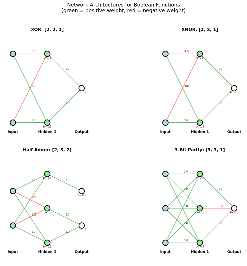
7. Network Architecture Exploration#
Let us build several small networks to compute different Boolean functions, exploring how architecture and weights determine function.
Show code cell source
# Collection of small networks for various Boolean functions

def test_network(net, name, X_test, y_test):
    """Test a network and print results."""
    n_inputs = X_test.shape[1]
    all_ok = True
    results = []
    for i in range(len(X_test)):
        pred = net.predict(X_test[i])
        pred_val = int(pred[0]) if len(pred) == 1 else tuple(int(p) for p in pred)
        target = int(y_test[i]) if np.isscalar(y_test[i]) else tuple(int(t) for t in y_test[i])
        ok = pred_val == target
        if not ok: all_ok = False
        results.append((X_test[i], pred_val, target, ok))

    print(f"\n{name}: {'PASS' if all_ok else 'FAIL'}")
    for x, pred, target, ok in results:
        x_str = ','.join(str(int(v)) for v in x)
        print(f"  ({x_str}) -> {pred}  (target: {target})  {'OK' if ok else 'FAIL'}")
    return all_ok


# All 2-input Boolean data
X2 = np.array([[0,0], [0,1], [1,0], [1,1]])

# 1. XOR
xor_net = MultiLayerNetwork([2, 2, 1])
xor_net.set_weights(0, [[1,1],[-1,-1]], [-0.5, 1.5])
xor_net.set_weights(1, [[1,1]], [-1.5])
test_network(xor_net, "XOR", X2, [0,1,1,0])

# 2. XNOR (complement of XOR)
xnor_net = MultiLayerNetwork([2, 2, 1])
xnor_net.set_weights(0, [[-1,-1],[1,1]], [1.5, -0.5])  # NAND, OR -> swap
xnor_net.set_weights(1, [[-1,-1]], [1.5])  # NAND of hidden
# Actually simpler: AND + NOR + OR
# h1 = AND(x1,x2) = step(x1+x2-1.5)
# h2 = NOR(x1,x2) = step(-x1-x2+0.5)
# y = OR(h1,h2) = step(h1+h2-0.5)
xnor_net2 = MultiLayerNetwork([2, 2, 1])
xnor_net2.set_weights(0, [[1,1],[-1,-1]], [-1.5, 0.5])
xnor_net2.set_weights(1, [[1,1]], [-0.5])
test_network(xnor_net2, "XNOR (AND + NOR + OR)", X2, [1,0,0,1])

# 3. Half Adder: computes (sum, carry) = (XOR, AND)
adder_net = MultiLayerNetwork([2, 3, 2])
# Hidden: OR, NAND, AND
adder_net.set_weights(0, [[1,1],[-1,-1],[1,1]], [-0.5, 1.5, -1.5])
# Output: XOR = AND(OR, NAND), Carry = AND (passthrough)
adder_net.set_weights(1, [[1,1,0],[0,0,1]], [-1.5, -0.5])

y_adder = np.array([[0,0], [1,0], [1,0], [0,1]])  # (sum, carry)
test_network(adder_net, "Half Adder (sum, carry)", X2, y_adder)

# 4. Majority-of-3
X3_all = np.array([[0,0,0],[0,0,1],[0,1,0],[0,1,1],[1,0,0],[1,0,1],[1,1,0],[1,1,1]])
y_maj3 = np.array([0,0,0,1,0,1,1,1])

# Majority of 3 is linearly separable! Single perceptron suffices.
# But let's show it can also be done with a hidden layer.
maj3_net = MultiLayerNetwork([3, 1])
maj3_net.set_weights(0, [[1,1,1]], [-1.5])  # step(x1+x2+x3-1.5)
test_network(maj3_net, "Majority-of-3 (single layer)", X3_all, y_maj3)
XOR: PASS
  (0,0) -> 0  (target: 0)  OK
  (0,1) -> 1  (target: 1)  OK
  (1,0) -> 1  (target: 1)  OK
  (1,1) -> 0  (target: 0)  OK

XNOR (AND + NOR + OR): PASS
  (0,0) -> 1  (target: 1)  OK
  (0,1) -> 0  (target: 0)  OK
  (1,0) -> 0  (target: 0)  OK
  (1,1) -> 1  (target: 1)  OK

Half Adder (sum, carry): PASS
  (0,0) -> (0, 0)  (target: (0, 0))  OK
  (0,1) -> (1, 0)  (target: (1, 0))  OK
  (1,0) -> (1, 0)  (target: (1, 0))  OK
  (1,1) -> (0, 1)  (target: (0, 1))  OK

Majority-of-3 (single layer): PASS
  (0,0,0) -> 0  (target: 0)  OK
  (0,0,1) -> 0  (target: 0)  OK
  (0,1,0) -> 0  (target: 0)  OK
  (0,1,1) -> 1  (target: 1)  OK
  (1,0,0) -> 0  (target: 0)  OK
  (1,0,1) -> 1  (target: 1)  OK
  (1,1,0) -> 1  (target: 1)  OK
  (1,1,1) -> 1  (target: 1)  OK
True
Show code cell source
# Visualize network architectures as diagrams

def draw_network(ax, layer_sizes, title, weights=None, biases=None):
    """Draw a simple network diagram."""
    n_layers = len(layer_sizes)
    max_neurons = max(layer_sizes)

    positions = {}  # (layer, neuron) -> (x, y)
    layer_names = ['Input'] + [f'Hidden {i+1}' for i in range(n_layers-2)] + ['Output']

    for l in range(n_layers):
        n = layer_sizes[l]
        x = l / (n_layers - 1) if n_layers > 1 else 0.5
        for j in range(n):
            y = (j - (n-1)/2) / max(max_neurons - 1, 1)
            positions[(l, j)] = (x, y)

    # Draw connections
    for l in range(n_layers - 1):
        for i in range(layer_sizes[l]):
            for j in range(layer_sizes[l+1]):
                x1, y1 = positions[(l, i)]
                x2, y2 = positions[(l+1, j)]
                w_val = weights[l][j, i] if weights else None

                if w_val is not None:
                    color = 'green' if w_val > 0 else ('red' if w_val < 0 else 'gray')
                    lw = min(abs(w_val) * 1.5, 4)
                else:
                    color = 'gray'
                    lw = 1

                ax.plot([x1, x2], [y1, y2], '-', color=color, linewidth=lw, alpha=0.6)

                if w_val is not None and abs(w_val) > 0.01:
                    mid_x = (x1 + x2) / 2 + 0.02
                    mid_y = (y1 + y2) / 2 + 0.02
                    ax.text(mid_x, mid_y, f'{w_val:.1f}', fontsize=7, color=color)

    # Draw neurons
    for l in range(n_layers):
        for j in range(layer_sizes[l]):
            x, y = positions[(l, j)]
            color = 'lightblue' if l == 0 else ('lightyellow' if l == n_layers-1 else 'lightgreen')
            circle = plt.Circle((x, y), 0.04, color=color, ec='black', linewidth=2, zorder=5)
            ax.add_patch(circle)

            # Bias label
            if biases and l > 0:
                b_val = biases[l-1][j]
                ax.text(x, y-0.07, f'b={b_val:.1f}', fontsize=7, ha='center', color='purple')

    # Layer labels
    for l in range(n_layers):
        x = l / (n_layers - 1) if n_layers > 1 else 0.5
        ax.text(x, -0.65, layer_names[l], fontsize=10, ha='center', fontweight='bold')

    ax.set_xlim(-0.15, 1.15)
    ax.set_ylim(-0.8, 0.8)
    ax.set_aspect('equal')
    ax.set_title(title, fontsize=12, fontweight='bold')
    ax.axis('off')


fig, axes = plt.subplots(2, 2, figsize=(14, 10))

# XOR network
draw_network(axes[0][0], [2, 2, 1], 'XOR: [2, 2, 1]',
             weights=[np.array([[1,1],[-1,-1]]), np.array([[1,1]])],
             biases=[np.array([-0.5, 1.5]), np.array([-1.5])])

# XNOR network
draw_network(axes[0][1], [2, 2, 1], 'XNOR: [2, 2, 1]',
             weights=[np.array([[1,1],[-1,-1]]), np.array([[1,1]])],
             biases=[np.array([-1.5, 0.5]), np.array([-0.5])])

# Half adder
draw_network(axes[1][0], [2, 3, 2], 'Half Adder: [2, 3, 2]',
             weights=[np.array([[1,1],[-1,-1],[1,1]]), np.array([[1,1,0],[0,0,1]])],
             biases=[np.array([-0.5, 1.5, -1.5]), np.array([-1.5, -0.5])])

# 3-bit parity
draw_network(axes[1][1], [3, 3, 1], '3-Bit Parity: [3, 3, 1]',
             weights=[np.ones((3,3)), np.array([[1,-1,1]])],
             biases=[np.array([-0.5, -1.5, -2.5]), np.array([-0.5])])

plt.suptitle('Network Architectures for Boolean Functions\n'
             '(green = positive weight, red = negative weight)',
             fontsize=14, y=1.02)
plt.tight_layout()
plt.show()
8. The Missing Piece: Learning#
In all the examples above, we designed the network weights by hand. We knew the target function and carefully chose weights to implement it. But in real applications:
We don’t know the target function exactly — we only have training examples.
We may not know the right architecture.
Manual weight design doesn’t scale to large networks.
We need a learning algorithm that can automatically find good weights from data.
The Perceptron Learning Rule Falls Short#
The perceptron learning rule (Chapter 5) can train a single-layer network:
But for multi-layer networks, the problem is the credit assignment problem: when the output is wrong, which hidden neuron’s weights should be adjusted, and by how much? The output error does not directly tell us how to update hidden-layer weights.
The Breakthrough: Backpropagation#
The solution is backpropagation (backward propagation of errors), which computes the gradient of the error with respect to every weight in the network by applying the chain rule of calculus layer by layer, from output to input.
Key dates:
1974: Paul Werbos describes backpropagation in his PhD thesis.
1986: Rumelhart, Hinton, and Williams publish the method in Nature, sparking the neural network renaissance.
The 17-Year Gap#
There is a remarkable 17-year gap between the publication of the limitations (Minsky and Papert, 1969) and the practical demonstration that multi-layer networks could overcome them (Rumelhart et al., 1986). During this period:
The multi-layer solution was known in principle but lacked a practical training algorithm.
Backpropagation existed (Werbos, 1974) but was not widely known or appreciated.
The AI community’s attention was elsewhere (expert systems, symbolic AI).
We will study backpropagation in detail in a later part of this course.
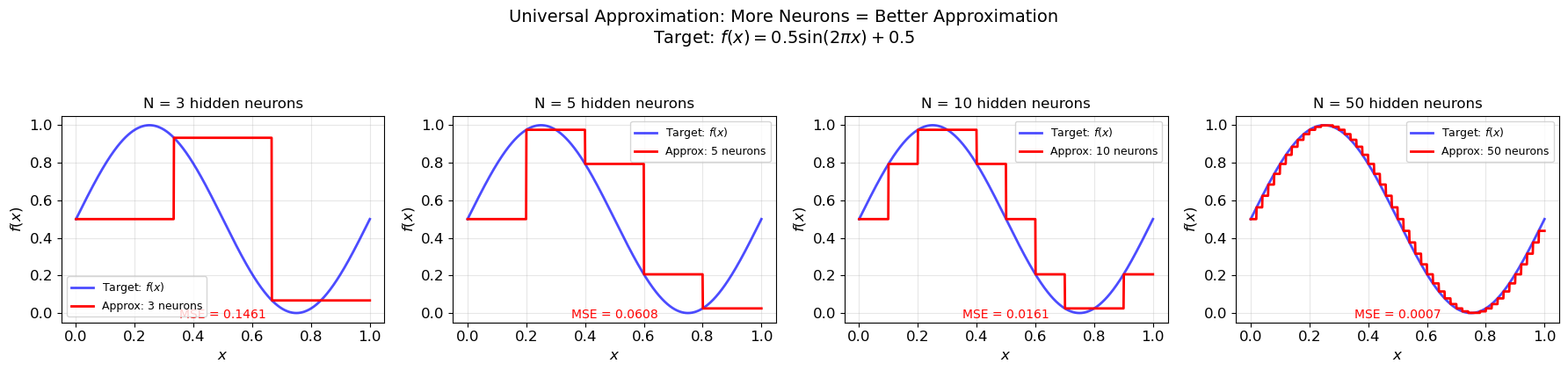
9. Universal Approximation Preview#
The multi-layer networks we have built solve specific Boolean functions. But how general is this approach? Can multi-layer networks approximate any function?
The Universal Approximation Theorem#
Theorem (Hornik, Stinchcombe, and White, 1989; Cybenko, 1989). Let \(\sigma\) be any non-constant, bounded, continuous activation function (e.g., sigmoid). Then for any continuous function \(f: [0,1]^n \to \mathbb{R}\) and any \(\epsilon > 0\), there exists a network with one hidden layer:
such that \(|F(\mathbf{x}) - f(\mathbf{x})| < \epsilon\) for all \(\mathbf{x} \in [0,1]^n\).
What This Says#
With enough hidden neurons, a single-hidden-layer network can approximate any continuous function to any desired accuracy. This is an existence theorem: it guarantees that the approximation is possible.
What This Does NOT Say#
The theorem leaves crucial questions unanswered:
How many neurons? The number \(N\) may be astronomically large.
Can we find the weights? The theorem proves existence but gives no algorithm.
Will the network generalize? Fitting training data perfectly doesn’t guarantee good performance on new data.
Are deeper networks more efficient? (Yes — this is one of the key motivations for deep learning.)
These questions drive much of modern neural network research.
Show code cell source
# Preview: universal approximation with step functions
# Approximate a smooth function using a hidden layer of step neurons

def sigmoid(z):
    return 1 / (1 + np.exp(-z))

def approx_function_step(x, n_neurons):
    """Approximate a function using n_neurons step-function hidden neurons.
    Uses evenly spaced thresholds to create a staircase approximation."""
    thresholds = np.linspace(0, 1, n_neurons + 1)[:-1]
    target = np.sin(2 * np.pi * x) * 0.5 + 0.5  # target function

    # Compute target values at thresholds
    target_at_thresholds = np.sin(2 * np.pi * thresholds) * 0.5 + 0.5

    # Weights: difference between consecutive target values
    output = np.zeros_like(x)
    for i in range(n_neurons):
        h = (x >= thresholds[i]).astype(float)
        if i == 0:
            weight = target_at_thresholds[0]
        else:
            weight = target_at_thresholds[i] - target_at_thresholds[i-1]
        output += weight * h

    return output


fig, axes = plt.subplots(1, 4, figsize=(18, 4))

x_plot = np.linspace(0, 1, 1000)
y_target = np.sin(2 * np.pi * x_plot) * 0.5 + 0.5

for idx, n_neurons in enumerate([3, 5, 10, 50]):
    ax = axes[idx]
    y_approx = approx_function_step(x_plot, n_neurons)

    ax.plot(x_plot, y_target, 'b-', linewidth=2, label='Target: $f(x)$', alpha=0.7)
    ax.plot(x_plot, y_approx, 'r-', linewidth=2, label=f'Approx: {n_neurons} neurons')
    ax.set_xlabel('$x$', fontsize=12)
    ax.set_ylabel('$f(x)$', fontsize=12)
    ax.set_title(f'N = {n_neurons} hidden neurons', fontsize=12)
    ax.legend(fontsize=9)
    ax.grid(True, alpha=0.3)

    # Compute error
    error = np.mean((y_target - y_approx)**2)
    ax.text(0.5, 0.02, f'MSE = {error:.4f}', transform=ax.transAxes,
            ha='center', fontsize=10, color='red')

plt.suptitle('Universal Approximation: More Neurons = Better Approximation\n'
             'Target: $f(x) = 0.5\\sin(2\\pi x) + 0.5$', fontsize=14, y=1.05)
plt.tight_layout()
plt.show()
10. Exercises#
Exercise 11.1: 3-Input Majority Function#
Design a network for the 3-input majority function:
Can you do it with a single perceptron (no hidden layer)? What are the weights?
Hint
Yes, the majority function is linearly separable! Try \(w_1 = w_2 = w_3 = 1\) and \(b = -1.5\). Then \(\text{step}(x_1 + x_2 + x_3 - 1.5) = 1\) whenever \(x_1 + x_2 + x_3 \geq 2\).
Exercise 11.3: “At Least 2 of 3” Function#
Design a network that computes the “at least 2 of 3” function:
Note: This is the same as the majority function! It is linearly separable, so a single perceptron suffices. Verify this.
Hint
Use weights \(w_1 = w_2 = w_3 = 1\) and bias \(b = -1.5\). The perceptron fires when \(x_1 + x_2 + x_3 \geq 1.5\), i.e., when at least 2 inputs are 1.
Exercise 11.4: XOR with Exactly 3 Neurons#
Can you solve XOR with a network of exactly 3 neurons total (2 hidden + 1 output)? We showed two constructions above that use exactly this architecture. Verify that 2 hidden neurons are necessary by proving that 1 hidden neuron is not sufficient.
Approach: A network with 1 hidden neuron has the form:
The hidden neuron maps \((x_1, x_2)\) to a single bit \(h \in \{0, 1\}\). The output neuron then makes a decision based on this single bit. But a single bit can only split the 4 input points into at most 2 groups. XOR requires distinguishing 3 groups (or showing that no partition into 2 groups works). Complete this argument.
Hint
The key insight: the hidden neuron computes some linearly separable function of \((x_1, x_2)\), producing a 1D output \(h \in \{0, 1\}\). The output neuron then applies a threshold to \(h\). So the output can either be \(h\) (identity) or \(1-h\) (negation). For the output to match XOR, we need \(h\) to be either XOR itself or XNOR — but neither is linearly separable. Contradiction!
Show code cell source
# Exercise 11.4: Proof that 1 hidden neuron is insufficient for XOR

print("Exhaustive search: can any 1-hidden-neuron network compute XOR?")
print("="*60)

X = np.array([[0,0], [0,1], [1,0], [1,1]])
y_xor = np.array([0, 1, 1, 0])

# A single hidden neuron computes h = step(w1*x1 + w2*x2 + b1)
# This partitions the 4 XOR inputs into two groups:
#   Group where h=0, and group where h=1

# There are only a limited number of possible partitions.
# For the output to compute XOR, we need:
#   All points with XOR=1 in one group, all with XOR=0 in the other.

# The possible partitions by a linear threshold on 2D:
# (which points have h=1?)

# Let's enumerate all possible h-assignments
from itertools import product

# For each of the 16 possible h-assignments
found_solution = False
print("\nFor each possible hidden neuron output pattern:")
print(f"{'h(0,0) h(0,1) h(1,0) h(1,1)':>30} | {'Can compute XOR?':>20}")
print("-" * 55)

for h_pattern in product([0, 1], repeat=4):
    h = np.array(h_pattern)
    # The output neuron sees only h (a single value)
    # It computes y = step(alpha * h + b2)
    # This means: either all h=0 map to one class and all h=1 to another,
    # or vice versa.

    # Case 1: output(h=0) = 0, output(h=1) = 1  => y = h
    y_pred_1 = h
    match_1 = np.array_equal(y_pred_1, y_xor)

    # Case 2: output(h=0) = 1, output(h=1) = 0  => y = 1-h
    y_pred_2 = 1 - h
    match_2 = np.array_equal(y_pred_2, y_xor)

    can_compute = match_1 or match_2

    # Check if this h_pattern is linearly separable (achievable by a single neuron)
    # (some patterns aren't, like XOR itself!)

    if can_compute:
        found_solution = True
        result = "YES"
    else:
        result = "no"

    h_str = f"  {h[0]}      {h[1]}      {h[2]}      {h[3]}"
    if can_compute:
        print(f"{h_str:>30} | {result:>20}  <-- CHECK IF REALIZABLE")

print("\nThe only h-patterns that could compute XOR are:")
print("  h = (0,1,1,0) with y=h, or h = (1,0,0,1) with y=1-h")
print("  But these ARE the XOR pattern itself!")
print("  A single neuron cannot compute XOR (Chapter 8).")
print("  Therefore: 1 hidden neuron is INSUFFICIENT.")
print()
print("CONCLUSION: XOR requires at least 2 hidden neurons. QED.")
Exhaustive search: can any 1-hidden-neuron network compute XOR?
============================================================

For each possible hidden neuron output pattern:
   h(0,0) h(0,1) h(1,0) h(1,1) |     Can compute XOR?
-------------------------------------------------------
        0      1      1      0 |                  YES  <-- CHECK IF REALIZABLE
        1      0      0      1 |                  YES  <-- CHECK IF REALIZABLE

The only h-patterns that could compute XOR are:
  h = (0,1,1,0) with y=h, or h = (1,0,0,1) with y=1-h
  But these ARE the XOR pattern itself!
  A single neuron cannot compute XOR (Chapter 8).
  Therefore: 1 hidden neuron is INSUFFICIENT.

CONCLUSION: XOR requires at least 2 hidden neurons. QED.