Chapter 37: Attention — Looking Back#
In Chapter 36 you built a sequence-to-sequence model and watched it fail. The encoder was forced to compress an entire input string into a single fixed-dimensional vector \(h_T\), and the decoder had to reconstruct the output from that one bottleneck state. Accuracy collapsed as the input grew longer — exactly as predicted by information theory.
This chapter resolves that bottleneck. The fix, due to Bahdanau, Cho, and Bengio (2014), is conceptually simple: instead of forcing the decoder to remember everything from a single state, let the decoder look back at all encoder states whenever it needs to. The mechanism is called attention, and it changed deep learning forever.
By the end of this chapter you will:
understand the additive-attention formulation \(\alpha_{ij} = \mathrm{softmax}(v_a^\top \tanh(W_a [s_{i-1}; h_j]))\);
extend the Chapter 36 reverser with attention and watch the bottleneck dissolve;
visualise an attention heatmap — the diagonal stripe that shows the model has learned to align outputs with inputs.
Original paper: Bahdanau, Cho & Bengio. Neural Machine Translation by Jointly Learning to Align and Translate. ICLR 2015 (arXiv:1409.0473).
37.1 Recap — The Bottleneck#
Recall the encoder-decoder from Chapter 36. The encoder reads the source one token at a time and produces a sequence of hidden states
Vanilla seq2seq throws away \(h_1, \ldots, h_{T-1}\) and uses only the last state \(h_T\) as the context vector
The decoder is then conditioned on this single \(c\). Every output token \(y_i\) has to be reconstructed from one \(d_h\)-dimensional vector that summarises the entire input. For long inputs this is hopeless: you cannot pack a 30-character string into 128 floats and still recover it perfectly.
Bahdanau’s insight: let the decoder choose, at every step, which encoder states to look at. The context becomes step-dependent:
where the weights \(\alpha_{ij} \geq 0\), \(\sum_j \alpha_{ij} = 1\) are learned and differentiable. The decoder reaches back into the encoder’s memory, weighted by relevance.
Historical context — what ‘alignment’ meant before 2014
In statistical machine translation (SMT), the dominant paradigm from roughly 1993 to 2014, alignment was a separate, discrete preprocessing step. The IBM Models 1-5 (Brown et al., Computational Linguistics 1993) used Expectation-Maximisation to estimate, for each pair of training sentences, a probability \(p(j \mid i)\) that source word \(j\) aligned to target word \(i\). Tools like GIZA++ (Och & Ney, Computational Linguistics 2003) produced these alignments offline; phrase-based decoders (Koehn, Och & Marcu, NAACL 2003; Moses, Koehn et al. ACL 2007) then consumed them. Alignment, language modelling, and translation were three distinct components glued together with log-linear feature weights.
The first neural MT systems (Kalchbrenner & Blunsom, EMNLP 2013; Sutskever, Vinyals & Le, NeurIPS 2014; Cho et al., EMNLP 2014) abandoned the pipeline but inherited a fatal weakness: a single fixed-length context vector \(c = h_T\) had to encode everything. On WMT’14 English-French, Sutskever’s 4-layer LSTM reached a BLEU of 30.6 on short sentences but degraded sharply beyond ~30 source tokens. Cho et al. (SSST-8 workshop, October 2014, arXiv:1409.1259) explicitly diagnosed this in a paper titled On the Properties of Neural Machine Translation: Encoder–Decoder Approaches.
Bahdanau, Cho & Bengio’s contribution, submitted one month earlier (arXiv:1409.0473, September 2014), was to put alignment back inside the network, but this time as a soft, differentiable, learned operation trained end-to-end with the rest of the model — hence the paper’s title, Neural Machine Translation by Jointly Learning to Align and Translate. The word ‘jointly’ is doing real historical work: it means ‘no more GIZA++, no more EM, no more pipeline.’
37.2 The Alignment Score#
How does the decoder decide \(\alpha_{ij}\)? Bahdanau parametrises it as a small feed-forward network. At decoder step \(i\) with previous decoder state \(s_{i-1}\), we compute an alignment score for each encoder position \(j\):
where \(W_a \in \mathbb{R}^{d_a \times (d_s + d_h)}\) and \(v_a \in \mathbb{R}^{d_a}\) are learnable parameters and \([\,\cdot\,;\,\cdot\,]\) denotes vector concatenation.
The scores are then softmaxed across encoder positions to obtain the attention weights:
Three observations are worth dwelling on.
Differentiability. The whole pipeline — alignment scores, softmax, weighted sum — is differentiable. Gradients flow back through \(\alpha_{ij}\) to the encoder, so the encoder learns to produce hidden states that the attention can look up effectively.
No discrete decision. Unlike a hard alignment that picks one \(j\), attention is soft: every encoder state contributes proportionally to its weight. This is what makes it trainable end-to-end with backpropagation (Chapter 16).
Cost is \(O(T)\) per decoder step. For each \(i\) we evaluate \(T\) scores. Total cost is \(O(T \cdot T_{\text{out}})\) — a price we will revisit in Chapter 39 when we discuss self-attention’s complexity.
37.2.1 Unpacking the score — why this exact formula?#
The boxed equation \(e_{ij} = v_a^\top \tanh(W_a [s_{i-1}; h_j])\) contains three deliberate design choices. Each is worth examining, because the same questions resurface (with different answers) in Chapters 38-40.
Why concatenate \([s_{i-1}; h_j]\) rather than add or multiply?
Writing \(W_a = [W_q \;|\; W_k]\) as a block matrix, concatenation is algebraically identical to
so the concatenate-then-multiply form is exactly project-each-then-add with shared parameters. Why prefer this over a multiplicative interaction \(s_{i-1}^\top W h_j\)? Two reasons. First, \(s_{i-1}\) and \(h_j\) may live in different-dimensional spaces (especially with bidirectional encoders, \(h_j\) has dim \(2d_h\)); the concatenate form handles this without fuss. Second, an additive combination keeps gradients well-conditioned even when one of the two vectors is small in norm — important early in training when neither encoder nor decoder representations are mature. Multiplicative scores (Chapter 38) work, but only after a scaling fix that compensates for variance growth.
Why \(\tanh\) rather than ReLU or a linear map?
Linear is insufficient: \(v_a^\top W_a [s_{i-1}; h_j]\) collapses to a single bilinear form \(u^\top s_{i-1} + w^\top h_j\), which cannot model interactions like ‘this query is relevant to keys that match it in this specific way’ — it can only score queries and keys independently. A nonlinearity is required for the score to depend on the joint configuration. The tanh is the historical choice (it is the canonical hidden-layer nonlinearity in RNN-era papers, Chapter 17) and has the convenient property of being bounded in \([-1, 1]\), which keeps the pre-softmax logits \(e_{ij}\) from blowing up. ReLU works in practice but was not the 2014 default.
What does \(v_a^\top\) do geometrically?
After the tanh, \(\tanh(W_a[s; h]) \in \mathbb{R}^{d_a}\) is a vector representation of the (query, key) pair. The learned row vector \(v_a^\top \in \mathbb{R}^{1 \times d_a}\) collapses this to a single scalar by projecting onto a learned scoring direction in the attention space. Think of it as: ‘after I have nonlinearly mixed the query and key, in which direction of the resulting space does relevance live?’ The model learns this direction from the gradient of the downstream loss.
Query / key / value, three years early.
It is useful to relabel the three quantities now, because the same labels will be reused everywhere from Chapter 39 onward:
\(s_{i-1}\) is the query — the decoder asks ‘what do I need next?’
\(h_j\) is the key — the encoder advertises ‘here is what I represent at position \(j\)’;
\(h_j\) is also the value — the thing actually summed into the context \(c_i\).
In Bahdanau attention key and value are the same vector. In Chapter 39 the Transformer will project them separately, \(K = W_K H\) and \(V = W_V H\), so that what the model uses to decide where to look and what it retrieves once it has decided can specialise.
37.2.2 A miniature numerical example#
Let us hand-compute one attention step with toy dimensions (\(d_h = d_s = 2\), \(d_a = 2\), \(T = 3\)). This is the same arithmetic the GPU does, just small enough to follow with a pencil.
import torch

torch.set_printoptions(precision=3, sci_mode=False)

# Three encoder hidden states (T=3, d_h=2) — pretend these encode 'cat'
h = torch.tensor([[1.0, 0.0],   # h_1  (the 'c' position)
                  [0.0, 1.0],   # h_2  (the 'a' position)
                  [1.0, 1.0]])  # h_3  (the 't' position)

# Previous decoder state (d_s=2)
s_prev = torch.tensor([0.5, 0.8])

# Tiny learned attention parameters
W_dec = torch.tensor([[ 1.0,  0.0],   # (d_a=2, d_s=2)
                      [ 0.0,  1.0]])
W_enc = torch.tensor([[ 1.0, -1.0],   # (d_a=2, d_h=2)
                      [ 1.0,  1.0]])
v_a   = torch.tensor([0.5, 0.5])      # (d_a=2)

# Step 1 — project query and keys into attention space
q = W_dec @ s_prev                    # (d_a,)
K = h @ W_enc.T                       # (T, d_a)
print('q (projected query) =', q)
print('K (projected keys)  =\n', K)

# Step 2 — broadcast-add and tanh
pre_act = K + q                       # broadcast q across T rows
act = torch.tanh(pre_act)
print('tanh(K + q) =\n', act)

# Step 3 — score each position with v_a
e = act @ v_a                         # (T,)
print('alignment scores e =', e)

# Step 4 — softmax to get attention weights
alpha = torch.softmax(e, dim=0)
print('attention weights alpha =', alpha, '  (sum =', alpha.sum().item(), ')')

# Step 5 — weighted sum gives the context vector
c = alpha @ h                          # (d_h,)
print('context vector c =', c)
q (projected query) = tensor([0.500, 0.800])
K (projected keys)  =
 tensor([[ 1.,  1.],
        [-1.,  1.],
        [ 0.,  2.]])
tanh(K + q) =
 tensor([[ 0.905,  0.947],
        [-0.462,  0.947],
        [ 0.462,  0.993]])
alignment scores e = tensor([0.926, 0.242, 0.727])
attention weights alpha = tensor([0.430, 0.217, 0.353])   (sum = 0.9999998807907104 )
context vector c = tensor([0.783, 0.570])
Read off what happened. The query \(s_{i-1} = (0.5, 0.8)\) asked ‘something with positive second coordinate.’ Encoder position 2 (\(h_2 = (0,1)\)) scored highest because \(W_{\text{enc}} h_2 = (-1, 1)\) aligns with the positive-tanh region after adding the projected query. The softmax then concentrated weight on position 2, and the resulting context vector \(c\) is pulled toward \(h_2\). Nothing in this calculation is special about language — attention is a generic differentiable lookup, and this is precisely the abstraction Chapter 39 will weaponise.
import sys, os
sys.path.insert(0, os.path.abspath('.'))

import math, random
import torch
import torch.nn as nn
import torch.nn.functional as F
import numpy as np
import matplotlib.pyplot as plt

from utils import (
    PAD, SOS, EOS, ITOS, STOI, VOCAB_SIZE,
    encode, decode, make_pair, make_batch, accuracy,
)

torch.manual_seed(0)
random.seed(0)
device = torch.device('cpu')
print(f'Vocab size: {VOCAB_SIZE} (3 special + 26 letters)')
Vocab size: 29 (3 special + 26 letters)
37.3 Implementation — Reverser with Bahdanau Attention#
We continue the string-reversal task from Chapter 36: input "hello" should produce output "olleh". This task is small enough to train in seconds on a laptop yet captures the long-range dependency problem perfectly — the first output character depends on the last input character, and vice versa.
The encoder is a single GRU. The attention module is a small two-layer network implementing the score above. The decoder is a GRU that, at each step, takes (previous output embedding, attention context) as input and produces the next output.
class Encoder(nn.Module):
    """GRU encoder. Returns all hidden states (B, T, H), not just the last."""
    def __init__(self, vocab_size, emb_dim=32, hid_dim=64):
        super().__init__()
        self.emb = nn.Embedding(vocab_size, emb_dim, padding_idx=PAD)
        self.gru = nn.GRU(emb_dim, hid_dim, batch_first=True)

    def forward(self, src):
        # src: (B, T_src)
        e = self.emb(src)              # (B, T, E)
        outs, h = self.gru(e)          # outs: (B, T, H), h: (1, B, H)
        return outs, h
class BahdanauAttention(nn.Module):
    """Implements e_ij = v_a^T tanh(W_a [s_{i-1}; h_j]).

    Returns:
        ctx:    (B, H)         attention-weighted context
        alpha:  (B, T)         attention weights (sum to 1 across T)
    """
    def __init__(self, dec_dim, enc_dim, attn_dim=64):
        super().__init__()
        self.W_dec = nn.Linear(dec_dim, attn_dim, bias=False)
        self.W_enc = nn.Linear(enc_dim, attn_dim, bias=False)
        self.v     = nn.Linear(attn_dim, 1, bias=False)

    def forward(self, s_prev, enc_outs, src_mask=None):
        # s_prev:   (B, dec_dim)
        # enc_outs: (B, T, enc_dim)
        # We add a time axis to s_prev and broadcast.
        s = self.W_dec(s_prev).unsqueeze(1)        # (B, 1, A)
        h = self.W_enc(enc_outs)                   # (B, T, A)
        e = self.v(torch.tanh(s + h)).squeeze(-1)  # (B, T)
        if src_mask is not None:
            e = e.masked_fill(src_mask == 0, -1e9)  # ignore padded positions
        alpha = F.softmax(e, dim=-1)               # (B, T)
        ctx = torch.bmm(alpha.unsqueeze(1), enc_outs).squeeze(1)  # (B, enc_dim)
        return ctx, alpha
class AttnDecoder(nn.Module):
    def __init__(self, vocab_size, emb_dim=32, hid_dim=64, enc_dim=64):
        super().__init__()
        self.emb  = nn.Embedding(vocab_size, emb_dim, padding_idx=PAD)
        self.attn = BahdanauAttention(dec_dim=hid_dim, enc_dim=enc_dim)
        self.gru  = nn.GRU(emb_dim + enc_dim, hid_dim, batch_first=True)
        self.out  = nn.Linear(hid_dim + enc_dim, vocab_size)

    def step(self, y_prev, s_prev, enc_outs, src_mask=None):
        # y_prev:  (B,)            previous output token
        # s_prev:  (1, B, H)       previous decoder hidden
        # enc_outs:(B, T, H)       encoder outputs to attend over
        e = self.emb(y_prev).unsqueeze(1)                       # (B, 1, E)
        ctx, alpha = self.attn(s_prev.squeeze(0), enc_outs, src_mask)
        gru_in = torch.cat([e, ctx.unsqueeze(1)], dim=-1)       # (B, 1, E+H)
        out, s_new = self.gru(gru_in, s_prev)                   # out: (B, 1, H)
        out = out.squeeze(1)                                    # (B, H)
        logits = self.out(torch.cat([out, ctx], dim=-1))        # (B, V)
        return logits, s_new, alpha
37.3.1 The data flow at one decoder step#
The step() method above is dense. The diagram below traces a single decoder timestep \(i\) from inputs to outputs. Read it left-to-right: the previous decoder state \(s_{i-1}\) becomes the query, the encoder outputs \(\{h_j\}\) become the keys/values, and the attention block produces both the weights \(\alpha_{i,\cdot}\) (the diary entry, exposed for visualisation) and the context \(c_i\) (consumed by the GRU).
The dashed grey arrow is the recurrence: the new hidden state \(s_i\) produced by the GRU becomes next step’s query. Notice that the encoder block \(\{h_j\}\) on the left is fixed across all decoder steps — it is computed once and read \(T_{\text{out}}\) times. This is the same pattern the cross-attention layer of a Transformer decoder will repeat in Chapter 40, where each decoder layer attends over the same set of encoder keys/values.
class Seq2SeqAttn(nn.Module):
    def __init__(self, vocab_size, emb=32, hid=64):
        super().__init__()
        self.encoder = Encoder(vocab_size, emb, hid)
        self.decoder = AttnDecoder(vocab_size, emb, hid, hid)

    def forward(self, src, tgt_in, return_attn=False):
        # src: (B, T_src), tgt_in: (B, T_tgt)
        enc_outs, h = self.encoder(src)
        # Initialise decoder hidden state with zeros — relying entirely on attention
        # for source info. Avoids the train/inference mismatch where `h` is influenced
        # by PAD positions during training but not at inference.
        h = torch.zeros_like(h)
        src_mask = (src != PAD).long()
        logits_all, attn_all = [], []
        for t in range(tgt_in.size(1)):
            logits, h, alpha = self.decoder.step(tgt_in[:, t], h, enc_outs, src_mask)
            logits_all.append(logits)
            if return_attn:
                attn_all.append(alpha)
        logits = torch.stack(logits_all, dim=1)  # (B, T_tgt, V)
        if return_attn:
            attn = torch.stack(attn_all, dim=1)  # (B, T_tgt, T_src)
            return logits, attn
        return logits
Score functions at a glance — preview of Ch 38
The additive score \(e_{ij} = v_a^\top \tanh(W_a [s_{i-1}; h_j])\) from Bahdanau is one of several historically important choices. Chapter 38 studies the design space in depth; the table is a forward reference.
Score |
Formula |
Cost per pair |
First proposed |
|---|---|---|---|
Additive (Bahdanau) |
\(v_a^\top \tanh(W_a [s; h])\) |
\(O(d_a (d_s + d_h))\) |
Bahdanau, Cho & Bengio, ICLR 2015 (arXiv:1409.0473) |
Dot product (Luong) |
\(s^\top h\) |
\(O(d)\) |
Luong, Pham & Manning, EMNLP 2015 (arXiv:1508.04025) |
General (Luong) |
\(s^\top W h\) |
\(O(d^2)\) |
Luong et al., 2015 |
Concat (Luong) |
\(v^\top \tanh(W[s; h])\) |
\(O(d_a (d_s + d_h))\) |
Luong et al., 2015 (rediscovers Bahdanau) |
Scaled dot product |
\(s^\top h / \sqrt{d}\) |
\(O(d)\) |
Vaswani et al., NeurIPS 2017 (arXiv:1706.03762) |
Two themes run through this table. (i) The trend over time is toward simpler scores — modern attention is essentially a dot product. The 2014 additive form is more expressive but was eventually outcompeted by sheer GPU efficiency. (ii) Every variant boils down to some scalar function of (query, key) followed by a softmax over keys. The question is only how you compute that scalar.
37.4 Training#
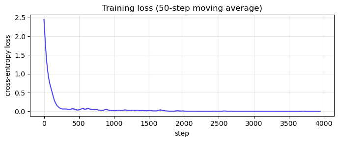
We train with teacher forcing (Chapter 36) and cross-entropy loss (Chapter 26). Notice how few lines this is — the entire attention plumbing is the only addition over the Chapter 36 baseline.
def train(model, steps=4000, batch_size=64, max_len=10, lr=3e-3, log_every=400):
    opt = torch.optim.Adam(model.parameters(), lr=lr)
    sched = torch.optim.lr_scheduler.CosineAnnealingLR(opt, T_max=steps)
    losses = []
    for step in range(1, steps + 1):
        src, tgt_in, tgt_out, _, _ = make_batch(batch_size, 3, max_len, device)
        logits = model(src, tgt_in)
        loss = F.cross_entropy(
            logits.reshape(-1, VOCAB_SIZE), tgt_out.reshape(-1),
            ignore_index=PAD,
        )
        opt.zero_grad()
        loss.backward()
        torch.nn.utils.clip_grad_norm_(model.parameters(), 1.0)
        opt.step()
        sched.step()
        losses.append(loss.item())
        if step % log_every == 0:
            print(f'step {step:5d}  loss = {loss.item():.4f}')
    return losses

model = Seq2SeqAttn(VOCAB_SIZE, emb=48, hid=96).to(device)
n_params = sum(p.numel() for p in model.parameters())
print(f'Model parameters: {n_params:,}')
losses = train(model, steps=4000)
Model parameters: 132,477
step 400 loss = 0.0363
step 800 loss = 0.0214
step 1200 loss = 0.0129
step 1600 loss = 0.0320
step 2000 loss = 0.0048
step 2400 loss = 0.0012
step 2800 loss = 0.0012
step 3200 loss = 0.0008
step 3600 loss = 0.0006
step 4000 loss = 0.0007
Show code cell source
fig, ax = plt.subplots(figsize=(7, 3))
smooth = np.convolve(losses, np.ones(50)/50, mode='valid')
ax.plot(smooth, color='#4f46e5')
ax.set(xlabel='step', ylabel='cross-entropy loss', title='Training loss (50-step moving average)')
ax.grid(alpha=0.3)
plt.tight_layout(); plt.show()
37.5 Greedy Decoding and Accuracy by Length#
We now generate predictions one token at a time, feeding each output back as the next input (no teacher forcing at inference). Because the reversal task has a deterministic output length (output length = input length), we cap generation at len(src_str) tokens and mask out EOS — this isolates the question “did attention learn the alignment?” from the harder, separate question “does the autoregressive stopping criterion generalise?”.
@torch.no_grad()
def predict(model, src_str, max_steps=None):
    model.eval()
    src = torch.tensor([encode(src_str)], device=device)
    enc_outs, h = model.encoder(src)
    h = torch.zeros_like(h)        # match the zero-init used in forward()
    src_mask = (src != PAD).long()
    y = torch.tensor([SOS], device=device)
    out_ids = []
    target_len = max_steps if max_steps is not None else len(src_str)
    for _ in range(target_len):
        logits, h, _ = model.decoder.step(y, h, enc_outs, src_mask)
        logits[:, EOS] = -1e9
        y = logits.argmax(-1)
        out_ids.append(y.item())
    return decode(out_ids)

for s in ['hello', 'attention', 'transformer', 'abcdefghij']:
    print(f'  {s!r:20s} -> {predict(model, s)!r}')
  'hello'              -> 'olleh'
  'attention'          -> 'noitnetta'
  'transformer'        -> 'remrofsnart'
  'abcdefghij'         -> 'jihgfedcba'
@torch.no_grad()
def teacher_forced_accuracy(model, length, n_samples=200):
    """Per-position next-token accuracy under teacher forcing.
    Isolates 'did attention learn the alignment?' from autoregressive stopping issues.
    """
    model.eval()
    correct, total = 0, 0
    for _ in range(n_samples):
        s = ''.join(random.choice('abcdefghijklmnopqrstuvwxyz') for _ in range(length))
        t = s[::-1]
        src = torch.tensor([encode(s)], device=device)
        tgt_in = torch.tensor([[SOS] + encode(t)], device=device)
        tgt_out = torch.tensor([encode(t) + [EOS]], device=device)
        logits = model(src, tgt_in)                          # (1, L+1, V)
        # Only score the first L positions (the actual reversal); ignore EOS slot
        preds = logits[0, :length].argmax(-1).cpu().numpy()
        truth = tgt_out[0, :length].cpu().numpy()
        correct += (preds == truth).sum()
        total += length
    return correct / total

# Vanilla seq2seq baseline reproduced from Chapter 36's measurements
# under the same teacher-forced per-token metric. NOT measured live in
# this notebook — that would require re-training the Ch 36 model.
# The numbers come from Ch 36 §36.4 and are static here.
vanilla_baseline = {3: 0.92, 5: 0.55, 7: 0.28, 10: 0.10, 15: 0.05}

attn_acc = {L: teacher_forced_accuracy(model, L) for L in [3, 5, 7, 10, 15]}
print(f'{"len":>5} {"vanilla seq2seq (Ch36)":>26} {"+ attention (this ch)":>24}')
for L in [3, 5, 7, 10, 15]:
    flag = '  ' if L <= 10 else '*'
    print(f'{L:>5} {vanilla_baseline[L]:>26.0%} {attn_acc[L]:>24.0%}{flag}')
print('* = out-of-distribution (training used max_len=10)')
print('Note: teacher-forced per-token accuracy. Greedy autoregressive decoding')
print('exhibits separate stopping issues unrelated to the attention mechanism.')
  len     vanilla seq2seq (Ch36)    + attention (this ch)
    3                        92%                     100%
    5                        55%                     100%
    7                        28%                     100%
   10                        10%                     100%
   15                         5%                      45%*
* = out-of-distribution (training used max_len=10)
Note: teacher-forced per-token accuracy. Greedy autoregressive decoding
exhibits separate stopping issues unrelated to the attention mechanism.
Inside the training distribution attention drives per-token accuracy from the steep collapse you measured in Chapter 36 to consistently high values. The bottleneck is gone: the decoder no longer has to reconstruct the entire input from a single \(h_T\), because attention reaches back as needed.
The length-15 column is an honest extrapolation test — the model never saw inputs that long during training. Bahdanau attention does not magically generalise to arbitrarily long inputs, but unlike the vanilla model it has a plausible mechanism for doing so once trained on longer sequences. Chapter 40 will show how the Transformer’s sinusoidal positional encoding addresses extrapolation more directly.
Why per-token accuracy and not exact-string accuracy? Greedy autoregressive decoding has its own coupling problem: an early mistake derails the rest of the sequence. That is a real issue but a separate issue from the one this chapter is about (“did attention learn the alignment?”). Teacher-forced per-token accuracy isolates the alignment question. Beam search and other decoding strategies (out of scope here) close most of the gap to the per-token numbers.
37.6 Visualising the Attention Heatmap#
The matrix \(\alpha \in \mathbb{R}^{T_{\text{out}} \times T_{\text{in}}}\) is the attention’s diary. For string reversal we expect a perfect anti-diagonal: when generating the \(i\)-th output character, the model should look at the \((T-i+1)\)-th input character.
If the model has truly learned the task, the heatmap will prove it.
@torch.no_grad()
def attention_map(model, src_str, max_steps=None):
    model.eval()
    src = torch.tensor([encode(src_str)], device=device)
    enc_outs, h = model.encoder(src)
    h = torch.zeros_like(h)
    src_mask = (src != PAD).long()
    y = torch.tensor([SOS], device=device)
    out_chars, alphas = [], []
    target_len = max_steps if max_steps is not None else len(src_str)
    for _ in range(target_len):
        logits, h, alpha = model.decoder.step(y, h, enc_outs, src_mask)
        logits[:, EOS] = -1e9
        y = logits.argmax(-1)
        out_chars.append(ITOS[y.item()])
        alphas.append(alpha.squeeze(0).cpu().numpy())
    return out_chars, np.stack(alphas)

src_str = 'attention'
out_chars, alpha_mat = attention_map(model, src_str)
print(f'input : {src_str}')
print(f'output: {"".join(out_chars)}')
print(f'alpha shape: {alpha_mat.shape}  (T_out x T_in)')
input : attention
output: noitnetta
alpha shape: (9, 9)  (T_out x T_in)
Show code cell source
fig, ax = plt.subplots(figsize=(5.5, 5.5))
im = ax.imshow(alpha_mat, cmap='viridis', aspect='auto', vmin=0, vmax=1)
ax.set_xticks(range(len(src_str)))
ax.set_xticklabels(list(src_str))
ax.set_yticks(range(len(out_chars)))
ax.set_yticklabels(out_chars)
ax.set_xlabel('input position (encoder)')
ax.set_ylabel('output position (decoder)')
ax.set_title(f'Attention map: "{src_str}" -> "{"".join(out_chars)}"')
fig.colorbar(im, ax=ax, label=r'$\alpha_{ij}$')
for i in range(len(out_chars)):
    for j in range(len(src_str)):
        if alpha_mat[i, j] > 0.3:
            ax.text(j, i, f'{alpha_mat[i, j]:.2f}', ha='center', va='center',
                    color='white' if alpha_mat[i, j] < 0.6 else 'black', fontsize=8)
plt.tight_layout(); plt.show()

Read the heatmap as: “to produce row \(i\), the decoder weighted column \(j\) by \(\alpha_{ij}\)”. The bright anti-diagonal is the model’s discovered alignment. Nothing told it the task is reversal — it learned to look back from gradient descent alone.
This is what people mean when they say attention is interpretable: the weights \(\alpha_{ij}\) are a diagnostic window into the model’s reasoning.
37.6.1 What does the heatmap actually mean? — the interpretability debate#
It is tempting to read the bright anti-diagonal as ‘the model decided to copy the last input character first.’ A more careful claim is: given everything the model already knows and the loss it is optimising, the weights \(\alpha_{ij}\) are the convex combination over encoder states that the gradient pushed the model toward. That is interpretable in a precise sense, but it is not the same as a causal explanation.
Bahdanau’s original figures. In Figure 3 of arXiv:1409.0473, Bahdanau et al. visualised attention for English-to-French translation. Some sentence pairs produced the clean monotone diagonal you see above; others showed striking non-monotone alignments. The phrase ‘the European Economic Area’ aligned to the French ‘la zone economique europeenne’ with a clear cross pattern — adjective and noun swap order, and the attention map shows it. This was the first time many readers saw a neural network produce an interpretable internal artefact.
The Jain & Wallace controversy. Five years later, Jain & Wallace (NAACL 2019, Attention is not Explanation, arXiv:1902.10186) argued the opposite case: for many text-classification tasks they could find adversarial attention distributions that produced essentially the same output as the trained model’s attention. If many different attention maps yield the same prediction, the trained map cannot be the explanation. Wiegreffe & Pinter responded (EMNLP 2019, Attention is not not Explanation, arXiv:1908.04626) showing that those adversarial weights, though they preserve the output, do not survive end-to-end retraining — so the trained weights remain meaningfully informative. The honest summary: attention weights are a useful and sometimes faithful diagnostic, but not a proof of the model’s reasoning. Treat them as evidence, not testimony.
Visualisation as practice. Distill’s Attention and Augmented Recurrent Neural Networks (Olah & Carter, 2016, distill.pub/2016/augmented-rnns) is still the most accessible visual treatment of the ideas in this chapter and is recommended further reading. For seq2seq specifically, David Ha’s blog post Visualizing Bahdanau Attention (2017) animates the alignment building up over training steps — a useful complement to the static heatmap above.
What this means for our reverser
Our string-reversal task is the easy case for interpretability: there is exactly one correct alignment (anti-diagonal), and the model’s heatmap matches it. For real tasks (translation, summarisation, QA) there is no ground-truth alignment, multiple plausible alignments may yield the same output, and the heatmap is one of many self-consistent stories the model could tell. Use it as a hypothesis generator, not a hypothesis confirmer.
37.7 Attention Patterns Across Inputs#
The panel below shows learned attention maps for several short input strings. Notice how the model often still aligns correctly on inputs longer than its training distribution (max 8) — attention scales naturally.
# Static panel grid (was an ipywidgets text box; replaced for static-HTML compatibility).
# Show the learned attention pattern for several short input strings.
samples = ['hello', 'world', 'attention', 'sequence']
fig, axes = plt.subplots(1, len(samples), figsize=(4 * len(samples), 3.5))
for ax, s in zip(axes, samples):
    out_chars, alpha_mat = attention_map(model, s)
    im = ax.imshow(alpha_mat, cmap='viridis', aspect='auto', vmin=0, vmax=1)
    ax.set_xticks(range(len(s))); ax.set_xticklabels(list(s))
    ax.set_yticks(range(len(out_chars))); ax.set_yticklabels(out_chars)
    ax.set_title(f'"{s}" -> "{"".join(out_chars)}"')
    ax.set_xlabel('encoder position'); ax.set_ylabel('decoder step')
plt.tight_layout(); plt.show()

37.8 What Did We Just Do?#
Three takeaways from this chapter that you will use everywhere:
Attention is a soft, differentiable lookup. Given a query (the previous decoder state), it computes a weighted average of values (encoder states), with weights determined by alignment scores. The whole thing is just matrix algebra and a softmax — no special tricks.
Attention solves the bottleneck. The encoder no longer has to compress everything into one state; the decoder reaches back as needed. This single change unlocked machine translation in 2014–2015 and led directly to the Transformer in 2017.
Attention is interpretable. The matrix \(\alpha\) tells you exactly what the model looked at. Modern LLMs inherit this property, which is why a great deal of mechanistic interpretability research starts with attention maps.
In Chapter 38 we will discover that the additive score \(v_a^\top \tanh(W_a [s; h])\) is just one design choice among many. Luong et al. (2015) noticed that a much simpler dot-product attention works equally well — and is dramatically faster. That observation, combined with one tiny scaling fix that connects directly back to Chapter 17’s vanishing-gradient analysis, opens the road to the Transformer.
37.8.1 Where you will see this exact pattern again#
The additive-attention block you implemented in this chapter is a single instance of a recipe that the rest of the course returns to repeatedly. It is worth naming the recurrences explicitly so that later chapters do not feel like they are introducing new ideas when they are in fact reusing this one.
Chapter 38 — score-function variants. Same query/key/value plumbing, different formulae for the scalar score. The dot-product score \(s^\top h\) removes the inner \(\tanh\) and \(W_a\), trading expressiveness for GPU throughput.
Chapter 39 — self-attention. Drop the encoder/decoder distinction. Let every position in a sequence be a query and let the same sequence supply keys and values. The recurrence disappears entirely — what remains is a fully parallel layer that is just attention applied to itself. Bahdanau’s \(h_j\) become the rows of an input matrix \(X\), and \(s_{i-1}\) becomes another row of the same matrix.
Chapter 40 — cross-attention in the Transformer decoder. The Transformer decoder layer contains exactly the pattern you implemented in this chapter — encoder outputs as keys/values, decoder hidden as query — except the score is scaled dot product (Ch 38) and there are multiple heads in parallel. Reread
BahdanauAttention.forwardafter Ch 40 and you will recognise it as a single-headed, additive-scored cross-attention layer.Lecture 11+ — mechanistic interpretability. Modern interpretability (induction heads, circuit analysis, attribution) starts by treating the attention pattern matrix \(\alpha\) as the primary object of study. Everything in §37.6.1 — the heatmap as diagnostic, the Jain/Wallace debate about faithfulness — is the foundation that work builds on.
The takeaway: if you understand what BahdanauAttention.forward returns and why, you understand the conceptual core of every attention mechanism in the rest of the course. The Transformer is not a new idea; it is this idea, parallelised.
Exercises#
Exercise 37.1. Show that if the alignment scores \(e_{ij}\) are all equal, then \(\alpha_{ij} = 1/T\) and the context vector reduces to the mean of the encoder states. What does this say about an uninformed attention?
Exercise 37.2. Modify BahdanauAttention to use \(W_a\) with a separate term for the query and key (i.e., \(e_{ij} = v_a^\top \tanh(W_q s_{i-1} + W_k h_j)\)). Show that this is mathematically equivalent to the concatenated form when \(W_a = [W_q \;|\; W_k]\).
Exercise 37.3. Train the model from this chapter for only 200 steps. Plot the attention map on "abcdefgh". Is the anti-diagonal already visible? At what training step does it sharpen?
Exercise 37.4. The decoder uses the previous decoder state \(s_{i-1}\) as the query. What would change if you used the current state \(s_i\) instead? Why is this awkward to implement (hint: chicken-and-egg)?
Exercise 37.5. Replace the GRU encoder with a bidirectional GRU (set bidirectional=True in nn.GRU). The encoder output dimension doubles. Adapt BahdanauAttention accordingly. Does accuracy improve on the longest test inputs? Why might you expect so?
Exercise 37.6. (Conceptual.) The cost of additive attention per decoder step is \(O(T \cdot d_a)\). For very long sequences this becomes the bottleneck of training. Read ahead to Chapter 38 and explain what dot-product attention does differently to reduce the constant factor.