Chapter 32: Sequences, Time, and Memory

Chapter 32: Sequences, Time, and Memory#

Every network we have studied so far processes its input in a single shot. A feedforward network receives a fixed-size vector, multiplies it by weight matrices layer by layer, and produces an output. The entire computation is memoryless: nothing about one input influences the processing of the next.

But what about data that unfolds over time? Speech, text, music – these are sequences where order matters and past context informs the present. A sentence is not a bag of words; a melody is not a set of notes. To handle sequences, we need networks with memory.

In this chapter we introduce recurrent neural networks (RNNs) – the first architecture designed to process sequential data. We trace the historical arc from Hopfield’s associative memory (1982) through Jordan’s and Elman’s recurrent architectures (1986, 1990), build an RNN cell from scratch in NumPy, verify it against PyTorch, and train a minimal next-character predictor.

Prerequisites

This chapter assumes familiarity with feedforward networks (Parts V–VI), backpropagation (Chapter 16), and basic PyTorch usage (Chapter 28).

Imports loaded: numpy, torch, matplotlib
PyTorch version: 2.7.0

32.1 Why Feedforward Networks Fail on Sequences#

Consider the task of classifying sentences by meaning. A feedforward network requires a fixed-size input, so the standard approach is bag-of-words: represent each sentence as a vector of word counts, ignoring order entirely.

This immediately reveals three fundamental problems:

Variable length. Sentences have different numbers of words. Padding to a maximum length wastes computation; truncating loses information.
Order dependence. “Dog bites man” and “Man bites dog” contain the same words, but mean very different things. A bag-of-words representation cannot distinguish them.
Long-range dependencies. In natural language, a word at position 50 can depend on a word at position 3 (e.g., subject-verb agreement across a long subordinate clause). Fixed-width windows cannot capture this.

Let us demonstrate problem (2) concretely.

# Demonstration: bag-of-words loses word order
vocab = {'dog': 0, 'bites': 1, 'man': 2, 'cat': 3, 'chases': 4, 'mouse': 5}
vocab_size = len(vocab)

def bag_of_words(sentence, vocab):
    """Convert sentence to a count vector."""
    bow = np.zeros(len(vocab))
    for word in sentence.lower().split():
        if word in vocab:
            bow[vocab[word]] += 1
    return bow

s1 = 'dog bites man'
s2 = 'man bites dog'
s3 = 'cat chases mouse'

bow1 = bag_of_words(s1, vocab)
bow2 = bag_of_words(s2, vocab)
bow3 = bag_of_words(s3, vocab)

print('Vocabulary:', vocab)
print()
print(f'"{s1}" -> {bow1}')
print(f'"{s2}" -> {bow2}')
print(f'"{s3}" -> {bow3}')
print()
print(f'Are "{s1}" and "{s2}" identical in BoW?  {np.array_equal(bow1, bow2)}')
print(f'Are "{s1}" and "{s3}" identical in BoW?  {np.array_equal(bow1, bow3)}')
print()
print('The bag-of-words representation CANNOT distinguish')
print('"dog bites man" from "man bites dog" -- a fatal flaw.')

Vocabulary: {'dog': 0, 'bites': 1, 'man': 2, 'cat': 3, 'chases': 4, 'mouse': 5}

"dog bites man" -> [1. 1. 1. 0. 0. 0.]
"man bites dog" -> [1. 1. 1. 0. 0. 0.]
"cat chases mouse" -> [0. 0. 0. 1. 1. 1.]

Are "dog bites man" and "man bites dog" identical in BoW?  True
Are "dog bites man" and "cat chases mouse" identical in BoW?  False

The bag-of-words representation CANNOT distinguish
"dog bites man" from "man bites dog" -- a fatal flaw.

Show code cell source Hide code cell source

# Train a simple MLP on bag-of-words to show it fails
# Task: classify as 0 = "agent acts on patient" vs 1 = "patient acts on agent"
# With BoW, s1 and s2 map to the same vector, so no MLP can separate them.

torch.manual_seed(42)

# Training data: 100 copies of each sentence with small noise
n_each = 100
X_train = []
y_train = []

rng = np.random.default_rng(42)
for _ in range(n_each):
    # "dog bites man" -> class 0
    X_train.append(bow1 + rng.normal(0, 0.05, vocab_size))
    y_train.append(0)
    # "man bites dog" -> class 1 (DIFFERENT meaning, SAME BoW)
    X_train.append(bow2 + rng.normal(0, 0.05, vocab_size))
    y_train.append(1)

X_train = torch.tensor(np.array(X_train), dtype=torch.float32)
y_train = torch.tensor(y_train, dtype=torch.long)

# Simple MLP
mlp = nn.Sequential(
    nn.Linear(vocab_size, 16),
    nn.ReLU(),
    nn.Linear(16, 2)
)

optimizer = torch.optim.Adam(mlp.parameters(), lr=0.01)
loss_fn = nn.CrossEntropyLoss()

losses = []
accs = []
for epoch in range(200):
    logits = mlp(X_train)
    loss = loss_fn(logits, y_train)
    optimizer.zero_grad()
    loss.backward()
    optimizer.step()
    
    preds = logits.argmax(dim=1)
    acc = (preds == y_train).float().mean().item()
    losses.append(loss.item())
    accs.append(acc)

fig, (ax1, ax2) = plt.subplots(1, 2, figsize=(11, 4))

ax1.plot(losses, color=BLUE, linewidth=1.5)
ax1.set_xlabel('Epoch')
ax1.set_ylabel('Cross-Entropy Loss')
ax1.set_title('MLP on Bag-of-Words: Loss', fontweight='bold')
ax1.axhline(y=np.log(2), color=RED, linestyle='--', label='Random baseline (ln 2)')
ax1.legend()

ax2.plot(accs, color=GREEN, linewidth=1.5)
ax2.set_xlabel('Epoch')
ax2.set_ylabel('Accuracy')
ax2.set_title('MLP on Bag-of-Words: Accuracy', fontweight='bold')
ax2.axhline(y=0.5, color=RED, linestyle='--', label='Chance level (50%)')
ax2.set_ylim(0, 1.05)
ax2.legend()

plt.tight_layout()
plt.show()

print(f'Final accuracy: {accs[-1]:.1%}')
print('The MLP cannot exceed 50% -- identical inputs have different labels.')
print('Word ORDER matters, but bag-of-words destroys it.')

../_images/97a0d215a8b26611d7462bcf65297a094562cbeaf82c2425cb92f75717125d89.png

Final accuracy: 50.5%
The MLP cannot exceed 50% -- identical inputs have different labels.
Word ORDER matters, but bag-of-words destroys it.

The Fundamental Limitation

A feedforward network operating on a bag-of-words representation is provably unable to distinguish inputs that differ only in word order. The sentences “dog bites man” and “man bites dog” map to identical feature vectors, so no function of those vectors can separate them. We need an architecture that processes words in sequence, maintaining a running state that encodes what has been seen so far.

32.2 Historical Arc#

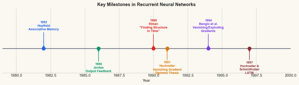
The idea of using recurrence – feeding a network’s own outputs back as inputs – has a rich history. Three milestones stand out.

Hopfield Networks (1982)#

John Hopfield’s seminal paper “Neural networks and physical systems with emergent collective computational abilities” (1982) introduced a network where every neuron is connected to every other neuron, with symmetric weights. The network’s dynamics converge to fixed points that serve as associative memories. While Hopfield networks are not sequence processors, they established the crucial concept that recurrent connections can store and retrieve information.

Jordan Networks (1986)#

Michael Jordan proposed a network architecture where the output at time \(t-1\) is fed back as additional input at time \(t\). This output-to-hidden feedback creates a simple form of memory: the network can use its own previous predictions to inform its current computation. Jordan networks were applied to sequential motor control tasks, demonstrating that recurrence enables temporal processing.

Elman Networks (1990)#

Jeffrey Elman’s landmark paper “Finding Structure in Time” (1990) introduced the architecture that became the standard simple recurrent network (SRN). The key innovation was hidden-to-hidden recurrence: instead of feeding back the output, the hidden state at time \(t-1\) is copied to a set of context units and used as additional input at time \(t\).

\[h_t = \sigma(W_h h_{t-1} + W_x x_t + b)\]

This seemingly small change had profound consequences: the hidden state becomes a learned internal representation of the sequence history, rather than a copy of the output. Elman demonstrated that his network could discover grammatical structure in simple artificial languages – learning to predict the next word in a sequence required implicitly learning the underlying grammar.

From Memory to Sequence Processing

The progression from Hopfield to Jordan to Elman represents a shift from static memory (fixed points) to dynamic memory (evolving hidden states). Hopfield networks remember patterns; Elman networks process sequences.

../_images/f87facd1d661d7df715b73a4ddb353995f87af184d825f138d97c4e542127b9f.png

32.3 The Simple RNN Cell#

The simple recurrent neural network (simple RNN, or SRN) processes a sequence \(x_1, x_2, \ldots, x_T\) one element at a time. At each time step \(t\), it combines the current input \(x_t\) with the previous hidden state \(h_{t-1}\) to produce a new hidden state \(h_t\).

Definition (Simple RNN Cell)

Given input \(x_t \in \mathbb{R}^d\), previous hidden state \(h_{t-1} \in \mathbb{R}^n\), and parameters \(W_x \in \mathbb{R}^{n \times d}\), \(W_h \in \mathbb{R}^{n \times n}\), \(b_h \in \mathbb{R}^n\), the simple RNN cell computes:

\[h_t = \tanh(W_h h_{t-1} + W_x x_t + b_h) \tag{RNN-1}\]

\[y_t = W_y h_t + b_y \tag{RNN-2}\]

where \(W_y \in \mathbb{R}^{m \times n}\), \(b_y \in \mathbb{R}^m\) are the output projection parameters, and \(h_0\) is typically initialized to \(\mathbf{0}\).

Two features distinguish the RNN from a feedforward network:

Recurrence. The hidden state \(h_t\) depends on \(h_{t-1}\), creating a chain of dependence reaching back to \(h_0\). This chain is the network’s memory.
Parameter sharing. The same weights \(W_x\), \(W_h\), \(W_y\) are used at every time step. This means the network can generalize across positions in the sequence (processing word 5 the same way as word 50), and it can handle sequences of any length without changing the number of parameters.

Why tanh?

The \(\tanh\) activation squashes the hidden state to \([-1, 1]\), preventing unbounded growth. Its derivative \(\tanh'(z) = 1 - \tanh^2(z)\) peaks at 1 (when \(z = 0\)) and decays toward 0 for large \(|z|\) – a property that will become important when we analyze gradient flow in Chapter 33.

../_images/ba3765962779c67929c592571a36425a3f1bdc813450874c2f685ad1b15d4163.png

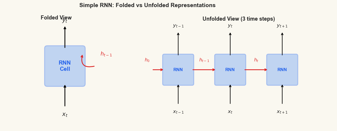
Left: the compact (folded) diagram with a self-loop for recurrence.
Right: the unfolded diagram showing the same weights applied at each step.
The red arrows carry the hidden state -- the network's memory.

32.4 Building an RNN from Scratch in NumPy#

Following the tradition of this course (cf. the McCullochPittsNeuron in Chapter 1, the Perceptron in Chapter 5, the NeuralNetwork in Chapter 18, and the Conv2D in Chapter 23), we implement the simple RNN cell from scratch in NumPy before reaching for any framework.

Our SimpleRNNCell class stores the weight matrices \(W_x\), \(W_h\), and bias \(b_h\), and implements a forward method that processes one input at a time, updating the hidden state.

class SimpleRNNCell:
    """A simple recurrent neural network cell (Elman RNN).
    
    Parameters
    ----------
    input_size : int
        Dimensionality of input vectors.
    hidden_size : int
        Dimensionality of the hidden state.
    seed : int
        Random seed for weight initialization.
    """
    def __init__(self, input_size, hidden_size, seed=42):
        self.input_size = input_size
        self.hidden_size = hidden_size
        
        # Xavier initialization
        rng = np.random.default_rng(seed)
        scale_x = np.sqrt(2.0 / (input_size + hidden_size))
        scale_h = np.sqrt(2.0 / (hidden_size + hidden_size))
        
        # W_x: input-to-hidden weights  (hidden_size x input_size)
        self.W_x = rng.normal(0, scale_x, (hidden_size, input_size))
        # W_h: hidden-to-hidden weights (hidden_size x hidden_size)
        self.W_h = rng.normal(0, scale_h, (hidden_size, hidden_size))
        # b_h: hidden bias
        self.b_h = np.zeros(hidden_size)
    
    def forward(self, x_t, h_prev):
        """Process one time step.
        
        Parameters
        ----------
        x_t : ndarray, shape (input_size,)
            Input at current time step.
        h_prev : ndarray, shape (hidden_size,)
            Hidden state from previous time step.
        
        Returns
        -------
        h_t : ndarray, shape (hidden_size,)
            New hidden state.
        """
        z = self.W_h @ h_prev + self.W_x @ x_t + self.b_h
        h_t = np.tanh(z)
        return h_t
    
    def forward_sequence(self, xs, h_init=None):
        """Process an entire sequence.
        
        Parameters
        ----------
        xs : ndarray, shape (T, input_size)
            Sequence of T input vectors.
        h_init : ndarray, shape (hidden_size,), optional
            Initial hidden state (default: zeros).
        
        Returns
        -------
        all_h : ndarray, shape (T, hidden_size)
            Hidden states at each time step.
        """
        if h_init is None:
            h_init = np.zeros(self.hidden_size)
        
        T = xs.shape[0]
        all_h = np.zeros((T, self.hidden_size))
        h = h_init
        
        for t in range(T):
            h = self.forward(xs[t], h)
            all_h[t] = h
        
        return all_h


print('SimpleRNNCell class defined.')
print('  h_t = tanh(W_h @ h_{t-1} + W_x @ x_t + b_h)')
print('  Methods: forward (one step), forward_sequence (full sequence)')

SimpleRNNCell class defined.
  h_t = tanh(W_h @ h_{t-1} + W_x @ x_t + b_h)
  Methods: forward (one step), forward_sequence (full sequence)

Let us hand-trace the RNN processing the string "hello". We encode each character as a one-hot vector and watch the hidden state evolve.

# Encode "hello" as one-hot vectors
text = 'hello'
chars = sorted(set(text))  # ['e', 'h', 'l', 'o']
char_to_idx = {c: i for i, c in enumerate(chars)}
idx_to_char = {i: c for c, i in char_to_idx.items()}

print(f'Text: "{text}"')
print(f'Vocabulary: {char_to_idx}')
print(f'Vocab size: {len(chars)}')
print()

# Create one-hot encoding
input_size = len(chars)
T = len(text)
xs = np.zeros((T, input_size))
for t, ch in enumerate(text):
    xs[t, char_to_idx[ch]] = 1.0

print('One-hot encodings:')
for t in range(T):
    print(f'  t={t}: "{text[t]}" -> {xs[t]}')

# Process with our RNN
hidden_size = 4  # small for readability
rnn_np = SimpleRNNCell(input_size=input_size, hidden_size=hidden_size, seed=42)

print(f'\nHidden size: {hidden_size}')
print(f'W_x shape: {rnn_np.W_x.shape}  (hidden x input)')
print(f'W_h shape: {rnn_np.W_h.shape}  (hidden x hidden)')
print(f'b_h shape: {rnn_np.b_h.shape}')
print()

# Hand-trace through the sequence
h = np.zeros(hidden_size)
print('--- Forward pass through "hello" ---')
print(f'h_0 = {h}')
for t in range(T):
    z = rnn_np.W_h @ h + rnn_np.W_x @ xs[t] + rnn_np.b_h
    h = np.tanh(z)
    print(f't={t} ("{text[t]}"): pre-activation z = [{" ".join(f"{v:+.3f}" for v in z)}]')
    print(f'           h_{t+1} = tanh(z) = [{" ".join(f"{v:+.3f}" for v in h)}]')

Text: "hello"
Vocabulary: {'e': 0, 'h': 1, 'l': 2, 'o': 3}
Vocab size: 4

One-hot encodings:
  t=0: "h" -> [0. 1. 0. 0.]
  t=1: "e" -> [1. 0. 0. 0.]
  t=2: "l" -> [0. 0. 1. 0.]
  t=3: "l" -> [0. 0. 1. 0.]
  t=4: "o" -> [0. 0. 0. 1.]

Hidden size: 4
W_x shape: (4, 4)  (hidden x input)
W_h shape: (4, 4)  (hidden x hidden)
b_h shape: (4,)

--- Forward pass through "hello" ---
h_0 = [0. 0. 0. 0.]
t=0 ("h"): pre-activation z = [-0.520 -0.651 -0.427 +0.564]
           h_1 = tanh(z) = [-0.478 -0.572 -0.402 +0.511]
t=1 ("e"): pre-activation z = [+0.149 -1.022 +0.181 -0.724]
           h_2 = tanh(z) = [+0.148 -0.771 +0.179 -0.619]
t=2 ("l"): pre-activation z = [+0.866 +0.470 +0.478 +0.416]
           h_3 = tanh(z) = [+0.699 +0.438 +0.445 +0.393]
t=3 ("l"): pre-activation z = [+0.480 +0.092 +0.403 +0.869]
           h_4 = tanh(z) = [+0.446 +0.091 +0.383 +0.701]
t=4 ("o"): pre-activation z = [+0.659 -0.051 +0.507 -0.051]
           h_5 = tanh(z) = [+0.578 -0.051 +0.468 -0.051]

Notice how the hidden state changes at every time step. After processing ‘h’, ‘e’, ‘l’, ‘l’, ‘o’, the final hidden state encodes (in a compressed form) the entire sequence history. The two ‘l’ characters produce different hidden states because the context (previous hidden state) differs.

Same Character, Different State

The letter ‘l’ appears twice in “hello” (at \(t=2\) and \(t=3\)), but the hidden states \(h_3\) and \(h_4\) are different. This is precisely because the RNN carries forward its memory: at \(t=2\), the context is “he”; at \(t=3\), the context is “hel”. A bag-of-characters model would treat both ‘l’s identically.

32.5 The Same RNN in PyTorch#

PyTorch provides nn.RNN as a built-in module. To verify that our NumPy implementation is correct, we initialize a PyTorch RNN with the same weights and confirm that the outputs match.

PyTorch RNN Convention

PyTorch’s nn.RNN returns two objects:

output: all hidden states, shape (seq_len, batch, hidden_size)
h_n: the final hidden state, shape (num_layers, batch, hidden_size)

By default, the input is expected in (seq_len, batch, input_size) format. PyTorch stores \(W_{ih}\) (our \(W_x\)) and \(W_{hh}\) (our \(W_h\)) as separate parameter matrices.

# Create PyTorch RNN and copy our NumPy weights into it
rnn_pt = nn.RNN(input_size=input_size, hidden_size=hidden_size,
                num_layers=1, nonlinearity='tanh', bias=True, batch_first=False)

# Copy weights from our NumPy RNN
with torch.no_grad():
    # PyTorch: weight_ih_l0 = W_x (hidden x input)
    rnn_pt.weight_ih_l0.copy_(torch.from_numpy(rnn_np.W_x).float())
    # PyTorch: weight_hh_l0 = W_h (hidden x hidden)
    rnn_pt.weight_hh_l0.copy_(torch.from_numpy(rnn_np.W_h).float())
    # PyTorch: bias_ih_l0 + bias_hh_l0 = b_h
    # PyTorch adds BOTH biases, so we put half in each
    rnn_pt.bias_ih_l0.copy_(torch.from_numpy(rnn_np.b_h / 2).float())
    rnn_pt.bias_hh_l0.copy_(torch.from_numpy(rnn_np.b_h / 2).float())

# Forward pass with PyTorch
xs_pt = torch.from_numpy(xs).float().unsqueeze(1)  # (T, 1, input_size)
h0_pt = torch.zeros(1, 1, hidden_size)             # (1, 1, hidden_size)

output_pt, hn_pt = rnn_pt(xs_pt, h0_pt)

# Our NumPy forward pass
all_h_np = rnn_np.forward_sequence(xs)

# Compare
print('Hidden states comparison (NumPy vs PyTorch):')
print(f'{"Step":<6} {"Char":<6} {"Max |difference|":<20}')
print('-' * 32)
for t in range(T):
    h_np = all_h_np[t]
    h_pt = output_pt[t, 0].detach().numpy()
    diff = np.max(np.abs(h_np - h_pt))
    print(f't={t:<4} "{text[t]}"    {diff:.2e}')

max_diff = np.max(np.abs(all_h_np - output_pt[:, 0].detach().numpy()))
print(f'\nMaximum absolute difference: {max_diff:.2e}')
print('Our NumPy implementation matches PyTorch!' if max_diff < 1e-6
      else 'WARNING: significant difference detected.')

Hidden states comparison (NumPy vs PyTorch):
Step   Char   Max |difference|    
--------------------------------
t=0    "h"    3.15e-08
t=1    "e"    6.09e-08
t=2    "l"    3.51e-08
t=3    "l"    5.31e-08
t=4    "o"    7.84e-08

Maximum absolute difference: 7.84e-08
Our NumPy implementation matches PyTorch!

32.6 Minimal Example: Next-Character Prediction#

Now we train a complete RNN model on a classic task: next-character prediction. Given a sequence of characters, predict the next character at each position. For example, given “hell”, predict “ello”.

We use the string "hello world" as our tiny training corpus. The model is deliberately small (hidden size 32, vocabulary of 8 unique characters) so it trains in seconds on the CPU.

Language Modeling

Next-character (or next-word) prediction is called language modeling. It is the foundation of modern NLP: GPT, the model behind ChatGPT, is fundamentally a next-token predictor trained on a massive corpus. Our tiny example here captures the same essential idea at the smallest possible scale.

# Next-character prediction on "hello world"
torch.manual_seed(42)

corpus = 'hello world'
chars_all = sorted(set(corpus))
vocab_size_lm = len(chars_all)
ch2i = {c: i for i, c in enumerate(chars_all)}
i2ch = {i: c for c, i in ch2i.items()}

print(f'Corpus: "{corpus}"')
print(f'Vocabulary ({vocab_size_lm} chars): {chars_all}')
print(f'Mapping: {ch2i}')

# Encode corpus as integer indices
encoded = [ch2i[c] for c in corpus]
print(f'Encoded: {encoded}')

# Create input/target pairs: input[t] -> target[t] = input[t+1]
x_indices = torch.tensor(encoded[:-1], dtype=torch.long)  # "hello worl"
y_indices = torch.tensor(encoded[1:], dtype=torch.long)   # "ello world"

print(f'\nInput:  {[i2ch[i.item()] for i in x_indices]}')
print(f'Target: {[i2ch[i.item()] for i in y_indices]}')

Corpus: "hello world"
Vocabulary (8 chars): [' ', 'd', 'e', 'h', 'l', 'o', 'r', 'w']
Mapping: {' ': 0, 'd': 1, 'e': 2, 'h': 3, 'l': 4, 'o': 5, 'r': 6, 'w': 7}
Encoded: [3, 2, 4, 4, 5, 0, 7, 5, 6, 4, 1]

Input:  ['h', 'e', 'l', 'l', 'o', ' ', 'w', 'o', 'r', 'l']
Target: ['e', 'l', 'l', 'o', ' ', 'w', 'o', 'r', 'l', 'd']

# Define the character-level RNN model
class CharRNN(nn.Module):
    """A minimal character-level language model using a simple RNN."""
    
    def __init__(self, vocab_size, hidden_size):
        super().__init__()
        self.hidden_size = hidden_size
        self.embedding = nn.Embedding(vocab_size, vocab_size)  # one-hot-like
        self.rnn = nn.RNN(vocab_size, hidden_size, batch_first=True)
        self.fc = nn.Linear(hidden_size, vocab_size)
        
        # Initialize embedding as identity (one-hot)
        with torch.no_grad():
            self.embedding.weight.copy_(torch.eye(vocab_size))
        self.embedding.weight.requires_grad = False  # freeze one-hot
    
    def forward(self, x, h=None):
        """Forward pass.
        
        Parameters
        ----------
        x : tensor, shape (batch, seq_len)
        h : tensor, shape (1, batch, hidden_size), optional
        
        Returns
        -------
        logits : tensor, shape (batch, seq_len, vocab_size)
        h_n : tensor, shape (1, batch, hidden_size)
        """
        emb = self.embedding(x)        # (batch, seq_len, vocab_size)
        out, h_n = self.rnn(emb, h)    # out: (batch, seq_len, hidden_size)
        logits = self.fc(out)           # (batch, seq_len, vocab_size)
        return logits, h_n


hidden_size_lm = 32
model = CharRNN(vocab_size_lm, hidden_size_lm)

n_params = sum(p.numel() for p in model.parameters() if p.requires_grad)
print(f'CharRNN model created.')
print(f'  Vocab size: {vocab_size_lm}')
print(f'  Hidden size: {hidden_size_lm}')
print(f'  Trainable parameters: {n_params}')
print(f'\nArchitecture:')
print(f'  Embedding({vocab_size_lm}) -> RNN({vocab_size_lm}, {hidden_size_lm}) -> Linear({hidden_size_lm}, {vocab_size_lm})')

CharRNN model created.
  Vocab size: 8
  Hidden size: 32
  Trainable parameters: 1608

Architecture:
  Embedding(8) -> RNN(8, 32) -> Linear(32, 8)

Show code cell source Hide code cell source

# Train the model
torch.manual_seed(42)
model = CharRNN(vocab_size_lm, hidden_size_lm)

optimizer = torch.optim.Adam(model.parameters(), lr=0.01)
loss_fn = nn.CrossEntropyLoss()

# Prepare data: single sequence, batch_size=1
x_train_lm = x_indices.unsqueeze(0)  # (1, seq_len)
y_train_lm = y_indices.unsqueeze(0)  # (1, seq_len)

n_epochs = 500
losses_lm = []
predictions_history = []

for epoch in range(n_epochs):
    model.train()
    logits, _ = model(x_train_lm)
    # logits: (1, seq_len, vocab_size), y: (1, seq_len)
    loss = loss_fn(logits.view(-1, vocab_size_lm), y_train_lm.view(-1))
    
    optimizer.zero_grad()
    loss.backward()
    optimizer.step()
    
    losses_lm.append(loss.item())
    
    if epoch in [0, 10, 50, 100, 200, 499]:
        preds = logits.argmax(dim=2)[0]
        pred_str = ''.join([i2ch[p.item()] for p in preds])
        predictions_history.append((epoch, pred_str, loss.item()))

# Plot training progress
fig, (ax1, ax2) = plt.subplots(1, 2, figsize=(12, 4.5))

ax1.plot(losses_lm, color=BLUE, linewidth=1.5)
ax1.set_xlabel('Epoch')
ax1.set_ylabel('Cross-Entropy Loss')
ax1.set_title('Training Loss', fontweight='bold')
ax1.set_yscale('log')
ax1.axhline(y=0, color=GRAY, linestyle='--', alpha=0.5)

# Show predictions at different epochs
ax2.axis('off')
target_str = ''.join([i2ch[y.item()] for y in y_indices])

table_data = [['Epoch', 'Predicted', 'Target', 'Loss']]
for epoch, pred_str, loss_val in predictions_history:
    table_data.append([str(epoch), pred_str, target_str, f'{loss_val:.3f}'])

table = ax2.table(cellText=table_data, loc='center', cellLoc='center')
table.auto_set_font_size(False)
table.set_fontsize(11)
table.scale(1.0, 1.8)

# Color header row
for j in range(4):
    table[0, j].set_facecolor(BLUE)
    table[0, j].set_text_props(color='white', fontweight='bold')

# Color correct/incorrect characters
for i in range(1, len(table_data)):
    pred = table_data[i][1]
    correct_count = sum(1 for a, b in zip(pred, target_str) if a == b)
    frac = correct_count / len(target_str)
    if frac == 1.0:
        table[i, 1].set_facecolor('#d1fae5')  # light green
    elif frac > 0.5:
        table[i, 1].set_facecolor('#fef3c7')  # light amber
    else:
        table[i, 1].set_facecolor('#fee2e2')  # light red

ax2.set_title('Predictions Over Training', fontweight='bold', fontsize=13)

fig.suptitle('Next-Character Prediction on "hello world"',
             fontsize=14, fontweight='bold')
plt.tight_layout()
plt.show()

print(f'Final loss: {losses_lm[-1]:.4f}')
print(f'The RNN learns to predict the next character in the sequence.')
print(f'Note: it learns "l" -> "l" AND "l" -> "o" by using context!')

../_images/444ad9a8db486e7abbe0af13951454b04436161e9ff5627454e08f41eafa4b54.png

Final loss: 0.0003
The RNN learns to predict the next character in the sequence.
Note: it learns "l" -> "l" AND "l" -> "o" by using context!

The Ambiguity of ‘l’

The character ‘l’ appears in two different contexts: after ‘e’ (where the next character is ‘l’) and after ‘l’ (where the next character is ‘o’). A model without memory would have to guess – it sees the same input ‘l’ and must produce two different outputs. The RNN resolves this ambiguity by using the hidden state: when processing the second ‘l’, it “remembers” that ‘l’ already appeared at the previous step, so it predicts ‘o’ instead of ‘l’.

Let us verify this by inspecting the hidden states when the model processes the two ‘l’ characters.

# Inspect hidden states for the two 'l' characters
model.eval()
with torch.no_grad():
    emb = model.embedding(x_train_lm)  # (1, seq_len, vocab_size)
    rnn_out, _ = model.rnn(emb)        # (1, seq_len, hidden_size)

# Positions of 'l' in the input "hello worl"
input_chars = [i2ch[i.item()] for i in x_indices]
l_positions = [i for i, c in enumerate(input_chars) if c == 'l']

print(f'Input sequence: {input_chars}')
print(f'Positions of "l": {l_positions}')
print()

for pos in l_positions:
    h_vec = rnn_out[0, pos].detach().numpy()
    logits_vec = model.fc(rnn_out[0, pos]).detach().numpy()
    probs = np.exp(logits_vec) / np.exp(logits_vec).sum()
    pred_char = i2ch[probs.argmax()]
    target_char = i2ch[y_indices[pos].item()]
    
    context = ''.join(input_chars[:pos+1])
    print(f'Position {pos}: input="l", context="{context}"')
    print(f'  Predicted: "{pred_char}" (correct: "{target_char}")')
    print(f'  Hidden state norm: {np.linalg.norm(h_vec):.3f}')
    print(f'  Top-3 probabilities: ', end='')
    top3 = np.argsort(probs)[::-1][:3]
    for idx in top3:
        print(f'"{i2ch[idx]}"={probs[idx]:.3f}  ', end='')
    print()

# Cosine similarity between hidden states at the two 'l' positions
h0 = rnn_out[0, l_positions[0]].detach().numpy()
h1 = rnn_out[0, l_positions[1]].detach().numpy()
cos_sim = np.dot(h0, h1) / (np.linalg.norm(h0) * np.linalg.norm(h1))
print(f'\nCosine similarity between h at pos {l_positions[0]} and pos {l_positions[1]}: {cos_sim:.3f}')
print('The hidden states are DIFFERENT despite the same input character.')
print('This is the power of recurrence: context shapes the hidden state.')

Input sequence: ['h', 'e', 'l', 'l', 'o', ' ', 'w', 'o', 'r', 'l']
Positions of "l": [2, 3, 9]

Position 2: input="l", context="hel"
  Predicted: "l" (correct: "l")
  Hidden state norm: 4.927
  Top-3 probabilities: "l"=1.000  "o"=0.000  "w"=0.000  
Position 3: input="l", context="hell"
  Predicted: "o" (correct: "o")
  Hidden state norm: 4.916
  Top-3 probabilities: "o"=1.000  "d"=0.000  " "=0.000  
Position 9: input="l", context="hello worl"
  Predicted: "d" (correct: "d")
  Hidden state norm: 5.097
  Top-3 probabilities: "d"=1.000  "o"=0.000  "l"=0.000  

Cosine similarity between h at pos 2 and pos 3: 0.251
The hidden states are DIFFERENT despite the same input character.
This is the power of recurrence: context shapes the hidden state.

Looking Ahead#

We have introduced the simple RNN and demonstrated that recurrence gives a network the ability to process sequences and maintain memory. But a critical question remains: how do we train these networks?

In Chapter 16, we derived backpropagation for feedforward networks by applying the chain rule layer by layer. For recurrent networks, the same principle applies – but the chain extends through time, creating dependencies that stretch back to the beginning of the sequence. This leads to backpropagation through time (BPTT), the subject of Chapter 33.

As we will discover, BPTT reveals a fundamental limitation of simple RNNs: gradients flowing backward through many time steps tend to either vanish (shrink to zero) or explode (grow without bound). This vanishing gradient problem – identified by Hochreiter (1991) and Bengio, Simard & Frasconi (1994) – motivated the invention of the LSTM architecture, which we will study in a subsequent chapter.

Exercises#

Exercise 32.1. Compute the number of trainable parameters in a simple RNN with input_size=10, hidden_size=64. Compare this to a feedforward network that processes a sequence of length \(T=20\) by concatenating all inputs into a single vector of size \(10 \times 20 = 200\) and mapping it to a hidden layer of 64 units. How does parameter count scale with sequence length in each architecture?

Exercise 32.2. Modify the SimpleRNNCell class to use the sigmoid activation instead of \(\tanh\). Trace through "hello" with the same weights and compare the hidden states. Why might \(\tanh\) be preferred over sigmoid for the hidden state update? (Hint: consider the range of the hidden state values.)

Exercise 32.3. A Jordan network feeds back the output rather than the hidden state. Write a JordanRNNCell class where the recurrence is \(h_t = \tanh(W_y y_{t-1} + W_x x_t + b_h)\), with \(y_t = W_o h_t + b_o\). Process "hello" and compare the hidden states to the Elman version.

Exercise 32.4. Train the CharRNN model on a longer string, such as "to be or not to be that is the question". How many epochs does it need to converge? What happens when you increase the hidden size from 32 to 64?

Exercise 32.5. The simple RNN uses \(\tanh(W_h h_{t-1} + W_x x_t + b)\) to compute the new hidden state. Show mathematically that if we remove the nonlinearity (i.e., use \(h_t = W_h h_{t-1} + W_x x_t + b\)), the hidden state after \(T\) steps is a linear function of all inputs \(x_1, \ldots, x_T\). Why does this make a linear RNN equivalent in expressiveness to a feedforward network? (Hint: expand the recurrence.)