Chapter 22: The Convolution Operation

Chapter 22: The Convolution Operation#

In Chapter 21, we motivated the need for convolutional neural networks by identifying three structural assumptions about image data: locality, weight sharing, and translation equivariance. In this chapter, we make these ideas precise by defining the convolution operation mathematically, implementing it in NumPy, and demonstrating its power as a feature extractor on synthetic images.

1. Cross-Correlation vs. Convolution#

In signal processing, convolution involves flipping the kernel before sliding it over the input. In deep learning, however, what we call “convolution” is actually cross-correlation—the kernel is applied without flipping. Since the network learns the kernel weights, flipping is irrelevant: the network simply learns the already-flipped version.

Warning: Naming Convention

Virtually all deep learning frameworks (TensorFlow, PyTorch, JAX) implement cross-correlation but call it “convolution.” We follow this convention throughout. When we say “convolution,” we mean cross-correlation unless explicitly stated otherwise.

Mathematical Definition#

Definition (2D Cross-Correlation / “Convolution”)

Given a 2D input \(\mathbf{X} \in \mathbb{R}^{H \times W}\) and a kernel \(\mathbf{K} \in \mathbb{R}^{K_h \times K_w}\), the 2D cross-correlation (with bias \(b\)) produces an output \(\mathbf{Y}\) where:

\[y_{i,j} = \sum_{u=0}^{K_h-1}\sum_{v=0}^{K_w-1} x_{i+u,\, j+v} \cdot k_{u,v} + b\]

for \(i = 0, 1, \ldots, H - K_h\) and \(j = 0, 1, \ldots, W - K_w\).

In words: place the kernel’s top-left corner at position \((i, j)\) in the input, compute the element-wise product of the kernel with the covered patch, sum all products, and add the bias. Repeat for every valid position.

For a true convolution, the kernel is first flipped both horizontally and vertically:

\[y_{i,j}^{\text{(true conv)}} = \sum_{u=0}^{K_h-1}\sum_{v=0}^{K_w-1} x_{i+u,\, j+v} \cdot k_{K_h - 1 - u,\, K_w - 1 - v} + b\]

Since learned kernels have no predefined orientation, the distinction is purely academic in the context of neural networks.

2. A 2D Convolution by Hand#

Let us work through a complete example. Consider a \(5 \times 5\) input and a \(3 \times 3\) kernel:

\[\begin{split}\mathbf{X} = \begin{pmatrix} 1 & 0 & 2 & 1 & 0 \\ 0 & 1 & 1 & 0 & 2 \\ 2 & 0 & 0 & 1 & 1 \\ 1 & 1 & 2 & 0 & 0 \\ 0 & 2 & 1 & 1 & 1 \end{pmatrix}, \quad \mathbf{K} = \begin{pmatrix} 1 & 0 & -1 \\ 1 & 0 & -1 \\ 1 & 0 & -1 \end{pmatrix}, \quad b = 0\end{split}\]

The output has size \((5 - 3 + 1) \times (5 - 3 + 1) = 3 \times 3\).

Position \((0, 0)\):

\[y_{0,0} = 1 \cdot 1 + 0 \cdot 0 + 2 \cdot (-1) + 0 \cdot 1 + 1 \cdot 0 + 1 \cdot (-1) + 2 \cdot 1 + 0 \cdot 0 + 0 \cdot (-1) = 1 - 2 - 1 + 2 = 0\]

Position \((0, 1)\):

\[y_{0,1} = 0 \cdot 1 + 2 \cdot 0 + 1 \cdot (-1) + 1 \cdot 1 + 1 \cdot 0 + 0 \cdot (-1) + 0 \cdot 1 + 0 \cdot 0 + 1 \cdot (-1) = -1 + 1 - 1 = -1\]

Continuing for all positions, we can verify the full result with the visualization below.

Show code cell source Hide code cell source

import numpy as np
import matplotlib.pyplot as plt
import matplotlib.patches as mpatches

plt.style.use('seaborn-v0_8-whitegrid')

# Define input and kernel
X = np.array([
    [1, 0, 2, 1, 0],
    [0, 1, 1, 0, 2],
    [2, 0, 0, 1, 1],
    [1, 1, 2, 0, 0],
    [0, 2, 1, 1, 1]
])

K = np.array([
    [1,  0, -1],
    [1,  0, -1],
    [1,  0, -1]
])

# Compute cross-correlation
kh, kw = K.shape
oh, ow = X.shape[0] - kh + 1, X.shape[1] - kw + 1
Y = np.zeros((oh, ow))
for i in range(oh):
    for j in range(ow):
        Y[i, j] = np.sum(X[i:i+kh, j:j+kw] * K)

def draw_matrix(ax, mat, title, cmap='Blues', highlight=None, fontsize=14):
    """Draw a matrix as a coloured grid with values."""
    h, w = mat.shape
    vmax = max(abs(mat.min()), abs(mat.max()), 1)
    ax.imshow(mat, cmap=cmap, vmin=-vmax, vmax=vmax, aspect='equal')
    for i in range(h):
        for j in range(w):
            color = 'white' if abs(mat[i, j]) > vmax * 0.6 else 'black'
            ax.text(j, i, f'{mat[i,j]:.0f}', ha='center', va='center',
                    fontsize=fontsize, fontweight='bold', color=color)
    if highlight is not None:
        r, c = highlight
        rect = mpatches.Rectangle((c - 0.5, r - 0.5), kw, kh,
                                   linewidth=3, edgecolor='#dc2626',
                                   facecolor='none', linestyle='--')
        ax.add_patch(rect)
    ax.set_title(title, fontsize=12, fontweight='bold')
    ax.set_xticks([])
    ax.set_yticks([])

fig, axes = plt.subplots(1, 3, figsize=(12, 4))

# Highlight position (0,0) in the input
draw_matrix(axes[0], X, 'Input X (5x5)', cmap='Blues', highlight=(0, 0))
draw_matrix(axes[1], K, 'Kernel K (3x3)', cmap='RdBu_r')
draw_matrix(axes[2], Y, 'Output Y (3x3)', cmap='RdBu_r')

# Highlight the (0,0) output position
rect = mpatches.Rectangle((-0.5, -0.5), 1, 1, linewidth=3,
                           edgecolor='#dc2626', facecolor='none', linestyle='--')
axes[2].add_patch(rect)

# Add operation symbols
fig.text(0.355, 0.5, '*', fontsize=28, ha='center', va='center', fontweight='bold')
fig.text(0.645, 0.5, '=', fontsize=28, ha='center', va='center', fontweight='bold')

plt.suptitle('2D Cross-Correlation ("Convolution")', fontsize=14, fontweight='bold', y=1.02)
plt.tight_layout()
plt.show()

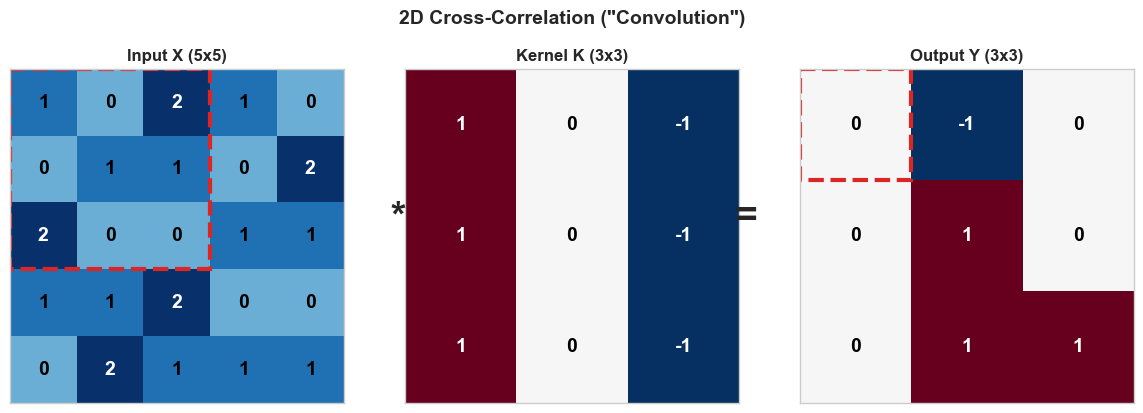
../_images/684c0ff5d2a975e7205a7043ea43fb7cacd2a5195640b58345e7cc69ee9adb66.png

Notice that this particular kernel is a vertical edge detector: it computes the difference between the left and right columns of each \(3 \times 3\) patch. Positive values in the output indicate left-to-right brightness transitions; negative values indicate right-to-left transitions.

3. Output Size Formula#

The output size depends on three parameters beyond the input and kernel sizes:

Padding \(P\): the number of zero-valued pixels added around the input border.
Stride \(S\): the step size when sliding the kernel.

Theorem (Output Size Formula)

For an input of spatial size \(W\), kernel size \(K\), padding \(P\), and stride \(S\):

\[\text{output\_size} = \left\lfloor \frac{W - K + 2P}{S} \right\rfloor + 1\]

The formula applies independently to height and width.

Special cases:

Configuration	Padding	Stride	Output Size
Valid (no padding)	\(P = 0\)	\(S = 1\)	\(W - K + 1\)
Same (preserve size)	\(P = \lfloor K/2 \rfloor\)	\(S = 1\)	\(W\)
Strided	\(P = 0\)	\(S > 1\)	\(\lfloor(W - K)/S\rfloor + 1\)

Worked Examples#

import numpy as np

def output_size(W, K, P=0, S=1):
    """Compute the output size of a convolution."""
    return (W - K + 2 * P) // S + 1

# Example 1: Valid convolution
print("Example 1: W=28, K=5, P=0, S=1")
print(f"  Output size: {output_size(28, 5, 0, 1)}")

# Example 2: Same padding
print("\nExample 2: W=28, K=5, P=2, S=1  ('same' padding)")
print(f"  Output size: {output_size(28, 5, 2, 1)}")

# Example 3: Stride 2
print("\nExample 3: W=28, K=5, P=0, S=2")
print(f"  Output size: {output_size(28, 5, 0, 2)}")

# Example 4: Stride 2 with padding
print("\nExample 4: W=32, K=3, P=1, S=2")
print(f"  Output size: {output_size(32, 3, 1, 2)}")

# Example 5: Large kernel
print("\nExample 5: W=224, K=7, P=3, S=2  (first layer of ResNet)")
print(f"  Output size: {output_size(224, 7, 3, 2)}")

Example 1: W=28, K=5, P=0, S=1
  Output size: 24

Example 2: W=28, K=5, P=2, S=1  ('same' padding)
  Output size: 28

Example 3: W=28, K=5, P=0, S=2
  Output size: 12

Example 4: W=32, K=3, P=1, S=2
  Output size: 16

Example 5: W=224, K=7, P=3, S=2  (first layer of ResNet)
  Output size: 112

Tip: “Same” Padding

To preserve the spatial dimensions with stride \(S=1\), set padding to \(P = \lfloor K/2 \rfloor\). For example, a \(3 \times 3\) kernel needs \(P = 1\); a \(5 \times 5\) kernel needs \(P = 2\). This is called “same” padding because the output has the same spatial size as the input.

4. Implementing Conv2D in NumPy#

We now implement a full Conv2D layer that handles multi-channel inputs, multiple output filters, and batched data. The input tensor has shape \((N, C_{\text{in}}, H, W)\) where \(N\) is the batch size and \(C_{\text{in}}\) is the number of input channels (e.g., 3 for RGB).

Each output filter has shape \((C_{\text{in}}, K, K)\)—it spans all input channels. With \(C_{\text{out}}\) filters, the weight tensor has shape \((C_{\text{out}}, C_{\text{in}}, K, K)\).

We use He initialization (Chapter 17), which sets the scale of initial weights to \(\sqrt{2 / \text{fan\_in}}\) where \(\text{fan\_in} = C_{\text{in}} \cdot K \cdot K\).

import numpy as np

class Conv2D:
    def __init__(self, in_channels, out_channels, kernel_size, seed=42):
        rng = np.random.default_rng(seed)
        fan_in = in_channels * kernel_size * kernel_size
        scale = np.sqrt(2.0 / fan_in)
        self.in_channels = in_channels
        self.out_channels = out_channels
        self.kernel_size = kernel_size
        self.weights = rng.normal(0.0, scale, size=(out_channels, in_channels, kernel_size, kernel_size))
        self.bias = np.zeros(out_channels)
    
    def forward(self, x):
        self.last_input = x
        batch_size, _, height, width = x.shape
        out_h = height - self.kernel_size + 1
        out_w = width - self.kernel_size + 1
        output = np.zeros((batch_size, self.out_channels, out_h, out_w))
        for row in range(out_h):
            for col in range(out_w):
                patch = x[:, :, row:row+self.kernel_size, col:col+self.kernel_size]
                output[:, :, row, col] = np.tensordot(patch, self.weights, axes=([1,2,3],[1,2,3])) + self.bias
        return output
    
    @property
    def parameter_count(self):
        return int(self.weights.size + self.bias.size)

# Verify our implementation
conv = Conv2D(in_channels=1, out_channels=4, kernel_size=3)
print(f"Weight shape: {conv.weights.shape}")
print(f"Bias shape:   {conv.bias.shape}")
print(f"Parameters:   {conv.parameter_count}")

# Test with a batch of 2 grayscale 8x8 images
x_test = np.random.default_rng(0).standard_normal((2, 1, 8, 8))
y_test = conv.forward(x_test)
print(f"\nInput shape:  {x_test.shape}")
print(f"Output shape: {y_test.shape}")
print(f"Expected:     (2, 4, 6, 6)")

Weight shape: (4, 1, 3, 3)
Bias shape:   (4,)
Parameters:   40

Input shape:  (2, 1, 8, 8)
Output shape: (2, 4, 6, 6)
Expected:     (2, 4, 6, 6)

Let us trace through the key line of the forward method:

output[:, :, row, col] = np.tensordot(patch, self.weights, axes=([1,2,3],[1,2,3])) + self.bias

patch has shape \((N, C_{\text{in}}, K, K)\)—the input region under the kernel for all batch elements.
self.weights has shape \((C_{\text{out}}, C_{\text{in}}, K, K)\).
tensordot with axes=([1,2,3],[1,2,3]) sums over channels \(\times\) kernel height \(\times\) kernel width, producing shape \((N, C_{\text{out}})\).
This is stored at spatial position \((\text{row}, \text{col})\) for all batch elements and all output channels simultaneously.

Note: Backward Pass

The Conv2D class above implements only the forward pass. The backward pass (computing gradients with respect to both the input and the kernel weights) will be derived in Chapter 24.

5. Edge Detection on Synthetic Patterns#

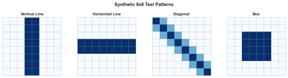
Before we let the network learn its own filters, let us see what hand-crafted kernels can do. We will create simple \(8 \times 8\) synthetic patterns and apply classical edge-detection kernels.

../_images/c2dbffa057a2a73982bfcbad0fc2b03549688b3a0202bfc04af63542ae3fd72c.png

Now we apply two classical edge-detection kernels:

Horizontal edge detector (detects horizontal boundaries):

\[\begin{split}\mathbf{K}_{\text{horiz}} = \begin{pmatrix} -1 & -1 & -1 \\ 0 & 0 & 0 \\ 1 & 1 & 1 \end{pmatrix}\end{split}\]

Vertical edge detector (detects vertical boundaries):

\[\begin{split}\mathbf{K}_{\text{vert}} = \begin{pmatrix} -1 & 0 & 1 \\ -1 & 0 & 1 \\ -1 & 0 & 1 \end{pmatrix}\end{split}\]

Show code cell source Hide code cell source

import numpy as np
import matplotlib.pyplot as plt

plt.style.use('seaborn-v0_8-whitegrid')

# Define edge detection kernels
K_horiz = np.array([[-1, -1, -1],
                    [ 0,  0,  0],
                    [ 1,  1,  1]], dtype=float)

K_vert = np.array([[-1, 0, 1],
                   [-1, 0, 1],
                   [-1, 0, 1]], dtype=float)

def cross_correlate_2d(image, kernel):
    """Simple 2D cross-correlation (no padding, stride=1)."""
    kh, kw = kernel.shape
    oh = image.shape[0] - kh + 1
    ow = image.shape[1] - kw + 1
    output = np.zeros((oh, ow))
    for i in range(oh):
        for j in range(ow):
            output[i, j] = np.sum(image[i:i+kh, j:j+kw] * kernel)
    return output

# Patterns to test
patterns = {
    'Vertical Line': make_vertical_line(),
    'Horizontal Line': make_horizontal_line(),
    'Diagonal': make_diagonal(),
    'Box': make_box(),
}

kernels = {
    'Horizontal Edge': K_horiz,
    'Vertical Edge': K_vert,
}

fig, axes = plt.subplots(len(kernels), len(patterns) + 1, figsize=(14, 6))

for ki, (kname, kernel) in enumerate(kernels.items()):
    # Show the kernel in the first column
    ax = axes[ki, 0]
    vmax = max(abs(kernel.min()), abs(kernel.max()))
    ax.imshow(kernel, cmap='RdBu_r', vmin=-vmax, vmax=vmax)
    for i in range(3):
        for j in range(3):
            ax.text(j, i, f'{kernel[i,j]:.0f}', ha='center', va='center',
                    fontsize=12, fontweight='bold',
                    color='white' if abs(kernel[i,j]) > 0.5 else 'black')
    ax.set_title(f'Kernel:\n{kname}', fontsize=10, fontweight='bold')
    ax.set_xticks([])
    ax.set_yticks([])
    
    # Apply kernel to each pattern
    for pi, (pname, pattern) in enumerate(patterns.items()):
        result = cross_correlate_2d(pattern, kernel)
        ax = axes[ki, pi + 1]
        vmax_r = max(abs(result.min()), abs(result.max()), 0.1)
        ax.imshow(result, cmap='RdBu_r', vmin=-vmax_r, vmax=vmax_r)
        ax.set_title(pname if ki == 0 else '', fontsize=10, fontweight='bold')
        ax.set_xticks([])
        ax.set_yticks([])
        # Add grid
        for i in range(result.shape[0] + 1):
            ax.axhline(i - 0.5, color='#94a3b8', linewidth=0.3)
        for j in range(result.shape[1] + 1):
            ax.axvline(j - 0.5, color='#94a3b8', linewidth=0.3)

plt.suptitle('Edge Detection: Kernel Responses to Synthetic Patterns',
             fontsize=13, fontweight='bold', y=1.02)
plt.tight_layout()
plt.show()

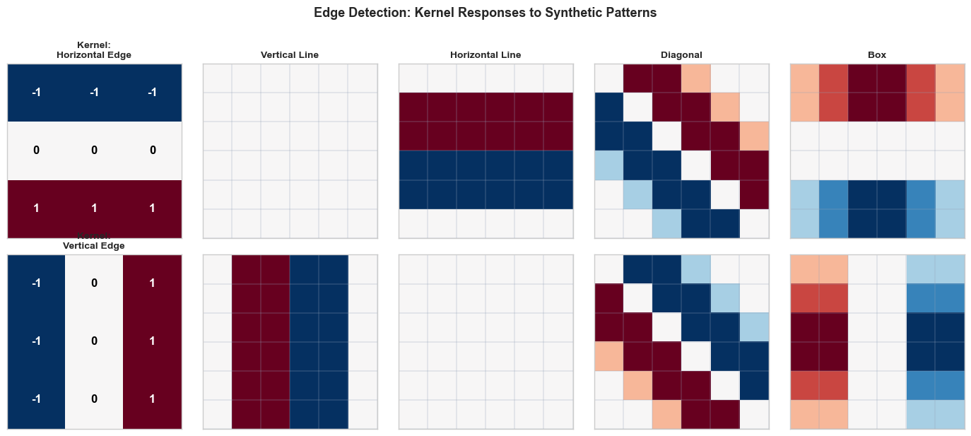
../_images/6fba7fabf564db20a89e3f8ba99d4b7f7f5c6b61183f57bdae24f0b766d82838.png

Observe the results:

The horizontal edge kernel produces strong responses on the horizontal line and the top/bottom edges of the box, but gives zero response on the vertical line (which has no horizontal gradients).
The vertical edge kernel lights up on the vertical line and the left/right edges of the box, but is blind to horizontal structures.
Both kernels respond to the diagonal, reflecting the fact that a diagonal edge has both horizontal and vertical components.

This is the essence of convolutional feature extraction: different kernels are sensitive to different spatial patterns. A CNN learns the right set of kernels for its task automatically through backpropagation.

Now let us use our Conv2D class with hand-crafted weights to verify it produces the same results:

# Use our Conv2D class with hand-crafted kernels
conv_edge = Conv2D(in_channels=1, out_channels=2, kernel_size=3)

# Manually set the kernels
conv_edge.weights[0, 0] = K_horiz  # First filter: horizontal edge
conv_edge.weights[1, 0] = K_vert   # Second filter: vertical edge
conv_edge.bias[:] = 0.0

# Create a batch with our test patterns
test_batch = np.stack([
    make_vertical_line(),
    make_horizontal_line(),
    make_box(),
])[:, np.newaxis, :, :]  # Shape: (3, 1, 8, 8)

output = conv_edge.forward(test_batch)
print(f"Input shape:  {test_batch.shape}  (batch=3, channels=1, 8x8)")
print(f"Output shape: {output.shape}  (batch=3, filters=2, 6x6)")
print(f"\nMax response of horiz-edge filter on horizontal line: {output[1, 0].max():.1f}")
print(f"Max response of vert-edge filter on vertical line:   {output[0, 1].max():.1f}")

Input shape:  (3, 1, 8, 8)  (batch=3, channels=1, 8x8)
Output shape: (3, 2, 6, 6)  (batch=3, filters=2, 6x6)

Max response of horiz-edge filter on horizontal line: 3.0
Max response of vert-edge filter on vertical line:   3.0

6. Multiple Filters and Channels#

In practice, a convolutional layer applies multiple filters to the input, each producing its own feature map. The collection of feature maps forms the layer’s output tensor.

Shape Conventions#

Throughout this course, we use the channels-first convention (NCHW):

Tensor	Shape	Description
Input	\((N, C_{\text{in}}, H, W)\)	Batch of \(N\) images, \(C_{\text{in}}\) channels
Weights	\((C_{\text{out}}, C_{\text{in}}, K, K)\)	\(C_{\text{out}}\) filters, each spanning all input channels
Bias	\((C_{\text{out}},)\)	One bias per output channel
Output	\((N, C_{\text{out}}, H_{\text{out}}, W_{\text{out}})\)	\(C_{\text{out}}\) feature maps

How Multi-Channel Convolution Works#

Each filter \(\bw_k \in \mathbb{R}^{C_{\text{in}} \times K \times K}\) produces one output feature map by:

Extracting a \((C_{\text{in}}, K, K)\) patch from the input at each spatial position.
Computing the dot product of this patch with the filter (summing over all channels and spatial positions within the kernel).
Adding the bias \(b_k\).

Definition (Feature Map)

A feature map is the 2D output produced by applying a single filter across all spatial positions of the input. If a convolutional layer has \(C_{\text{out}}\) filters, it produces \(C_{\text{out}}\) feature maps, which together form the output tensor.

../_images/3a9ffe3a720ee450f09c64a9d64777d5260df482eeada0506047c9442743068c.png

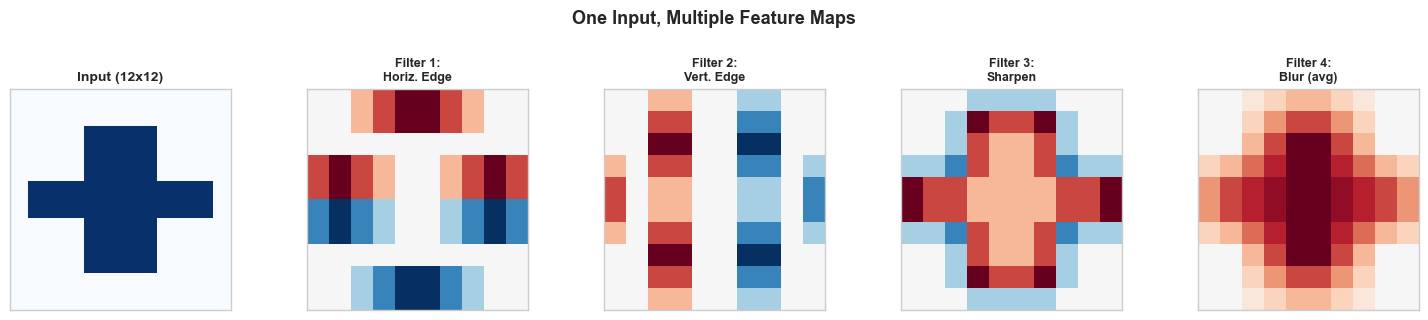
Each filter extracts a different aspect of the input:

The horizontal edge filter highlights the top and bottom boundaries of the cross shape.
The vertical edge filter highlights the left and right boundaries.
The sharpening filter enhances contrast at all edges.
The averaging (blur) filter smooths the image, reducing noise.

In a trained CNN, the network discovers which filters are useful for the task at hand. Early layers typically learn edge detectors and texture filters; deeper layers learn more complex patterns like corners, shapes, and eventually parts of objects.

Parameter Count#

The total number of learnable parameters in a Conv2D layer is:

\[\text{params} = C_{\text{out}} \times (C_{\text{in}} \times K \times K + 1)\]

where the \(+1\) accounts for one bias per filter. This is independent of the input spatial dimensions \(H\) and \(W\)—one of the key advantages of convolution over fully connected layers.

7. Exercises#

Exercise 22.1: Convolution by Hand#

Compute the full output of the following convolution (no padding, stride 1, no bias):

\[\begin{split}\mathbf{X} = \begin{pmatrix} 2 & 1 & 0 & 3 \\ 1 & 0 & 2 & 1 \\ 0 & 3 & 1 & 0 \\ 1 & 2 & 0 & 1 \end{pmatrix}, \quad \mathbf{K} = \begin{pmatrix} 1 & -1 \\ -1 & 1 \end{pmatrix}\end{split}\]

Verify that the output has shape \(3 \times 3\) and compute all 9 values.

Exercise 22.2: Output Size Computation#

For each configuration, compute the output spatial dimensions:

(a) Input: \(32 \times 32\), Kernel: \(5 \times 5\), Padding: 0, Stride: 1

(b) Input: \(32 \times 32\), Kernel: \(5 \times 5\), Padding: 2, Stride: 1

(d) Input: \(224 \times 224\), Kernel: \(11 \times 11\), Padding: 2, Stride: 4 (AlexNet first layer)

(e) Input: \(7 \times 7\), Kernel: \(3 \times 3\), Padding: 1, Stride: 1. How many times can you apply this operation while maintaining the same spatial size?

Exercise 22.3: Parameter Comparison#

Consider processing a \(64 \times 64 \times 3\) RGB input.

(a) Compute the number of parameters in a fully connected layer that maps this input to 64 output units.

(b) Compute the number of parameters in a Conv2D layer with 64 filters of size \(3 \times 3\) applied to the same input.

Exercise 22.4: Identity Kernel#

What \(3 \times 3\) kernel acts as the identity (output equals input, assuming valid padding)? Test your answer by applying it to a \(5 \times 5\) input matrix.

Exercise 22.5: Implementing Stride#

Extend the Conv2D class to support a stride parameter. The constructor should accept stride=1 by default. Modify the forward method so that the kernel moves by stride pixels at each step. Verify that:

With stride 1 on an \(8 \times 8\) input with \(3 \times 3\) kernel, the output is \(6 \times 6\).
With stride 2 on an \(8 \times 8\) input with \(3 \times 3\) kernel, the output is \(3 \times 3\).

Hint: The main change is in the loop bounds and indexing:

for row in range(out_h):
    for col in range(out_w):
        patch = x[:, :, row*stride:row*stride+self.kernel_size,
                        col*stride:col*stride+self.kernel_size]

8. Summary and Key Takeaways#

In deep learning, “convolution” actually refers to cross-correlation: the kernel is not flipped before sliding.
The output of a 2D convolution at position \((i, j)\) is: \(y_{i,j} = \sum_{u,v} x_{i+u,j+v} \cdot k_{u,v} + b\).
The output size formula is \(\lfloor(W - K + 2P)/S\rfloor + 1\), where \(W\) is input size, \(K\) is kernel size, \(P\) is padding, and \(S\) is stride.
Our Conv2D class implements forward propagation with He initialization and supports batched, multi-channel inputs.
Hand-crafted kernels (horizontal/vertical edge detectors) demonstrate that convolution is a natural operation for feature extraction.
Multiple filters produce multiple feature maps, each sensitive to different spatial patterns.
Convolutional layers have far fewer parameters than equivalent fully connected layers, and the count is independent of input spatial size.

9. References#

Y. LeCun, L. Bottou, Y. Bengio, and P. Haffner, “Gradient-based learning applied to document recognition,” Proceedings of the IEEE, vol. 86, no. 11, pp. 2278–2324, 1998.
I. Goodfellow, Y. Bengio, and A. Courville, Deep Learning, MIT Press, 2016. Chapter 9: Convolutional Networks.
A. Krizhevsky, I. Sutskever, and G. E. Hinton, “ImageNet classification with deep convolutional neural networks,” Advances in Neural Information Processing Systems, vol. 25, 2012.