Chapter 2: Building Logic from Neurons

Chapter 2: Building Logic from Neurons#

1. Introduction: From Gates to Circuits#

In Chapter 1, we saw that a single McCulloch-Pitts neuron can compute any threshold function — a Boolean function that outputs 1 when a weighted sum of inputs exceeds a fixed threshold. The canonical examples are AND (\(\theta = 2\)), OR (\(\theta = 1\)), and NOT (with an inhibitory input and a bias).

But we also saw that not every Boolean function is a threshold function. XOR — the exclusive-or — is the simplest counterexample. To compute XOR and, more generally, arbitrary Boolean functions, we need to compose neurons into networks.

This chapter explores three progressively deeper results:

The DNF Construction Algorithm: A systematic procedure to build a feedforward M-P network for any Boolean function, given its truth table.
XOR as a warning sign: The impossibility of computing XOR with a single neuron is the first hint of the deeper linear separability constraint that will return to haunt the field in 1969.
Feedforward vs. Recurrent Networks: When we allow cycles in the network, M-P neurons can implement memory and state machines. McCulloch and Pitts proved that recurrent networks are equivalent to finite automata (their Theorem II), and argued (informally) for a connection to Turing machines.
The key limitation: Despite their computational power, M-P networks have no mechanism for learning. Every connection is hardwired. This limitation will motivate Hebb (1949), Rosenblatt (1958), and the entire learning-theoretic tradition.

We begin by bringing forward the McCullochPittsNeuron and McCullochPittsNetwork classes from Chapter 1.

Tip

This chapter demonstrates a fundamental pattern in computer science: simple components composed systematically can produce arbitrarily complex behavior. A single M-P neuron is limited, but networks of M-P neurons are universal. This same principle applies to transistors (simple switches that compose into CPUs), to NAND gates (a single universal gate), and later to artificial neurons with learned weights.

import numpy as np
import matplotlib.pyplot as plt
from itertools import product
%matplotlib inline


class McCullochPittsNeuron:
    """A McCulloch-Pitts neuron (reproduced from Chapter 1)."""

    def __init__(self, threshold, name=None):
        if threshold < 1:
            raise ValueError("Threshold must be a positive integer.")
        self.threshold = threshold
        self.name = name or f"MP(theta={threshold})"

    def activate(self, excitatory_inputs, inhibitory_inputs=None):
        if inhibitory_inputs is not None and any(inhibitory_inputs):
            return 0
        excitatory_sum = sum(excitatory_inputs)
        return 1 if excitatory_sum >= self.threshold else 0

    def __repr__(self):
        return f"McCullochPittsNeuron(threshold={self.threshold}, name='{self.name}')"


class McCullochPittsNetwork:
    """A feedforward network of McCulloch-Pitts neurons (reproduced from Chapter 1)."""

    def __init__(self, n_inputs):
        self.n_inputs = n_inputs
        self.layers = []

    def add_layer(self, layer_spec):
        self.layers.append(layer_spec)

    def forward(self, inputs):
        if len(inputs) != self.n_inputs:
            raise ValueError(f"Expected {self.n_inputs} inputs, got {len(inputs)}")
        current_signals = list(inputs)
        for layer in self.layers:
            next_signals = []
            for spec in layer:
                neuron = spec['neuron']
                exc = [current_signals[i] for i in spec['excitatory']]
                inh = [current_signals[i] for i in spec['inhibitory']]
                output = neuron.activate(exc, inh)
                next_signals.append(output)
            current_signals = next_signals
        return current_signals

    def __repr__(self):
        desc = f"McCullochPittsNetwork(inputs={self.n_inputs}, layers={len(self.layers)})"
        for i, layer in enumerate(self.layers):
            neurons = [s['neuron'].name for s in layer]
            desc += f"\n  Layer {i}: {neurons}"
        return desc


print("Classes loaded successfully.")

Classes loaded successfully.

2. The DNF Construction Algorithm#

Theory#

Recall from Chapter 1 that any Boolean function \(f: \{0,1\}^n \to \{0,1\}\) can be expressed in Disjunctive Normal Form (DNF):

\[f(x_1, \ldots, x_n) = \bigvee_{\mathbf{a} \in f^{-1}(1)} \left( \bigwedge_{i=1}^{n} \ell_i^{(\mathbf{a})} \right)\]

where \(\ell_i^{(\mathbf{a})} = x_i\) if \(a_i = 1\) and \(\ell_i^{(\mathbf{a})} = \neg x_i\) if \(a_i = 0\).

Theorem (DNF Universality)

Every Boolean function \(f: \{0,1\}^n \to \{0,1\}\) can be expressed in Disjunctive Normal Form, and therefore can be realized by a feedforward McCulloch-Pitts network with at most three layers (negation, conjunction, disjunction) using at most \(n + 2^n + 1\) neurons.

The algorithm to convert a truth table into an M-P network is:

Extract minterms: Identify all input patterns \(\mathbf{a}\) where \(f(\mathbf{a}) = 1\).
Build negation layer: Create NOT neurons (with bias) for each input variable.
Build minterm layer: For each minterm, create an AND neuron (threshold \(= n\)) whose excitatory inputs are the appropriate literals (\(x_i\) or \(\neg x_i\)).
Build output layer: Create an OR neuron (threshold \(= 1\)) that takes all minterm outputs as excitatory inputs.

Warning

Exponential blowup of the DNF construction. The DNF construction is universal but can be astronomically expensive. For a Boolean function on \(n\) inputs, the truth table has \(2^n\) rows, and the DNF may require up to \(2^n\) minterm neurons (one for each row where \(f = 1\)). For \(n = 20\), that is over 1 million neurons; for \(n = 30\), over 1 billion. In practice, most Boolean functions of interest have much more compact representations — but the DNF construction does not exploit any such structure. Finding minimal networks is, in general, an NP-hard problem.

Implementation#

Show code cell source Hide code cell source

def boolean_to_mp_network(truth_table, n_vars):
    """Convert a Boolean function (truth table) into a feedforward M-P network using DNF."""
    minterms = [inp for inp, out in truth_table.items() if out == 1]

    if len(minterms) == 0:
        net = McCullochPittsNetwork(n_vars + 1)
        net.add_layer([
            {'neuron': McCullochPittsNeuron(n_vars + 2, 'ZERO'),
             'excitatory': list(range(n_vars)),
             'inhibitory': []}
        ])
        return net

    bias_idx = n_vars
    net = McCullochPittsNetwork(n_vars + 1)

    layer1 = []
    for i in range(n_vars):
        layer1.append({
            'neuron': McCullochPittsNeuron(1, f'NOT_x{i}'),
            'excitatory': [bias_idx],
            'inhibitory': [i]
        })
    for i in range(n_vars):
        layer1.append({
            'neuron': McCullochPittsNeuron(1, f'PASS_x{i}'),
            'excitatory': [i],
            'inhibitory': []
        })
    net.add_layer(layer1)

    layer2 = []
    for m_idx, minterm in enumerate(minterms):
        exc_indices = []
        for i in range(n_vars):
            if minterm[i] == 1:
                exc_indices.append(n_vars + i)
            else:
                exc_indices.append(i)
        layer2.append({
            'neuron': McCullochPittsNeuron(n_vars, f'MINT_{minterm}'),
            'excitatory': exc_indices,
            'inhibitory': []
        })
    net.add_layer(layer2)

    layer3 = [
        {
            'neuron': McCullochPittsNeuron(1, 'OR_out'),
            'excitatory': list(range(len(minterms))),
            'inhibitory': []
        }
    ]
    net.add_layer(layer3)

    return net


def verify_network(net, truth_table, n_vars):
    """Verify that a network (with bias) computes the given truth table."""
    all_pass = True
    header = " ".join([f"x{i}" for i in range(n_vars)]) + "  expected  got  status"
    print(header)
    print("-" * len(header))
    for inputs, expected in sorted(truth_table.items()):
        full_input = list(inputs) + [1]
        result = net.forward(full_input)[0]
        status = "PASS" if result == expected else "FAIL"
        if result != expected:
            all_pass = False
        vals = " ".join([f"{v:>2}" for v in inputs])
        print(f"{vals}  {expected:>8}  {result:>3}  {status}")
    return all_pass


print("DNF construction algorithm defined.")

DNF construction algorithm defined.

==================================================
Example 1: AND(x0, x1) via DNF construction
==================================================
McCullochPittsNetwork(inputs=3, layers=3)
  Layer 0: ['NOT_x0', 'NOT_x1', 'PASS_x0', 'PASS_x1']
  Layer 1: ['MINT_(1, 1)']
  Layer 2: ['OR_out']

  AND(0, 0) = 0  (expected 0)  [PASS]
  AND(0, 1) = 0  (expected 0)  [PASS]
  AND(1, 0) = 0  (expected 0)  [PASS]
  AND(1, 1) = 1  (expected 1)  [PASS]

==================================================
Example 2: MAJORITY(x0, x1, x2) via DNF construction
==================================================
McCullochPittsNetwork(inputs=4, layers=3)
  Layer 0: ['NOT_x0', 'NOT_x1', 'NOT_x2', 'PASS_x0', 'PASS_x1', 'PASS_x2']
  Layer 1: ['MINT_(0, 1, 1)', 'MINT_(1, 0, 1)', 'MINT_(1, 1, 0)', 'MINT_(1, 1, 1)']
  Layer 2: ['OR_out']

  MAJ(0, 0, 0) = 0  (expected 0)  [PASS]
  MAJ(0, 0, 1) = 0  (expected 0)  [PASS]
  MAJ(0, 1, 0) = 0  (expected 0)  [PASS]
  MAJ(0, 1, 1) = 1  (expected 1)  [PASS]
  MAJ(1, 0, 0) = 0  (expected 0)  [PASS]
  MAJ(1, 0, 1) = 1  (expected 1)  [PASS]
  MAJ(1, 1, 0) = 1  (expected 1)  [PASS]
  MAJ(1, 1, 1) = 1  (expected 1)  [PASS]

==================================================
Example 3: IMPLIES(x0, x1) = NOT x0 OR x1
==================================================
McCullochPittsNetwork(inputs=3, layers=3)
  Layer 0: ['NOT_x0', 'NOT_x1', 'PASS_x0', 'PASS_x1']
  Layer 1: ['MINT_(0, 0)', 'MINT_(0, 1)', 'MINT_(1, 1)']
  Layer 2: ['OR_out']

  IMP(0, 0) = 1  (expected 1)  [PASS]
  IMP(0, 1) = 1  (expected 1)  [PASS]
  IMP(1, 0) = 0  (expected 0)  [PASS]
  IMP(1, 1) = 1  (expected 1)  [PASS]

3. XOR: The First Warning Sign#

The Impossibility Result#

Definition (Exclusive-OR)

The exclusive-or function is defined as:

\[\begin{split}\text{XOR}(x_1, x_2) = \begin{cases} 1 & \text{if } x_1 \neq x_2 \\ 0 & \text{if } x_1 = x_2 \end{cases}\end{split}\]

Danger

XOR cannot be computed by a single McCulloch-Pitts neuron.

This is a fundamental limitation. No matter how you assign inputs to excitatory/inhibitory roles, and no matter what threshold you choose, a single M-P neuron cannot produce the XOR truth table. This is because:

A single M-P neuron computes a threshold function (with absolute inhibition).
XOR is not a threshold function.
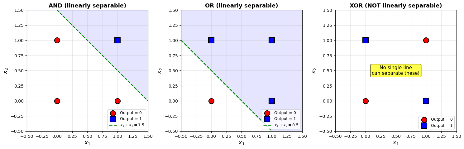
Equivalently, the positive examples \(\{(0,1), (1,0)\}\) and negative examples \(\{(0,0), (1,1)\}\) of XOR are not linearly separable.

This seemingly minor observation foreshadows the crisis that nearly killed the field: Minsky and Papert’s Perceptrons (1969) generalized this result to show that single-layer networks cannot compute many important functions (parity, connectedness, etc.).

Theorem. No single McCulloch-Pitts neuron can compute XOR.

Proof. A single M-P neuron computes a function of the form:

\[\begin{split}y = \begin{cases} 1 & \text{if } \displaystyle\sum_{j \in E} x_j \geq \theta \text{ and } \sum_{k \in I} x_k = 0 \\ 0 & \text{otherwise} \end{cases}\end{split}\]

The key property is monotonicity in excitatory inputs: if all inhibitory inputs are 0, then adding more active excitatory inputs can only increase (or maintain) the likelihood of firing.

For XOR, we need \(f(0,1) = f(1,0) = 1\) but \(f(1,1) = 0\). If both inputs are excitatory, then \(f(1,0) = 1\) implies \(\theta \leq 1\). But then \(f(1,1)\): the excitatory sum is \(2 \geq 1 = \theta\), so \(f(1,1) = 1\). Contradiction.

If we try making one input inhibitory (say \(x_2\)), then \(f(0, 1) = 0\) (since \(x_2\) is inhibitory and active), but we need \(f(0,1) = 1\). Contradiction.

No assignment of roles (excitatory/inhibitory) to the two inputs, for any threshold, produces the XOR truth table. \(\blacksquare\)

Geometric Interpretation#

Definition (Linear Separability)

A Boolean function \(f: \{0,1\}^n \to \{0,1\}\) is linearly separable if there exists a hyperplane in \(\mathbb{R}^n\) that separates the points where \(f = 1\) from the points where \(f = 0\). Formally, there exist weights \(w_1, \ldots, w_n\) and a threshold \(\theta\) such that:

\[f(\mathbf{x}) = 1 \iff \sum_{i=1}^{n} w_i x_i \geq \theta\]

This result has a beautiful geometric explanation. A single threshold neuron partitions input space with a hyperplane. In 2D, a line. The XOR function’s positive examples \(\{(0,1), (1,0)\}\) and negative examples \(\{(0,0), (1,1)\}\) are not linearly separable — no single line can separate them.

Show code cell source Hide code cell source

# --- Visualization: Why XOR is not linearly separable ---
import numpy as np
import matplotlib.pyplot as plt
%matplotlib inline

fig, axes = plt.subplots(1, 3, figsize=(15, 5))

for ax in axes:
    ax.set_xlim(-0.5, 1.5)
    ax.set_ylim(-0.5, 1.5)
    ax.set_xlabel('$x_1$', fontsize=13)
    ax.set_ylabel('$x_2$', fontsize=13)
    ax.set_aspect('equal')
    ax.grid(True, alpha=0.3)

x_line = np.linspace(-0.5, 1.5, 100)

# --- AND ---
ax = axes[0]
ax.set_title('AND (linearly separable)', fontsize=13, fontweight='bold')
ax.scatter([0, 0, 1], [0, 1, 0], c='red', s=150, zorder=5,
           edgecolors='black', linewidth=1.5, label='Output = 0')
ax.scatter([1], [1], c='blue', s=150, zorder=5, marker='s',
           edgecolors='black', linewidth=1.5, label='Output = 1')
ax.plot(x_line, 1.5 - x_line, 'g--', linewidth=2, label='$x_1 + x_2 = 1.5$')
ax.fill_between(x_line, 1.5 - x_line, 1.5, alpha=0.1, color='blue')
ax.legend(loc='lower right', fontsize=9)

# --- OR ---
ax = axes[1]
ax.set_title('OR (linearly separable)', fontsize=13, fontweight='bold')
ax.scatter([0], [0], c='red', s=150, zorder=5,
           edgecolors='black', linewidth=1.5, label='Output = 0')
ax.scatter([0, 1, 1], [1, 0, 1], c='blue', s=150, zorder=5, marker='s',
           edgecolors='black', linewidth=1.5, label='Output = 1')
ax.plot(x_line, 0.5 - x_line, 'g--', linewidth=2, label='$x_1 + x_2 = 0.5$')
ax.fill_between(x_line, 0.5 - x_line, 1.5, alpha=0.1, color='blue')
ax.legend(loc='lower right', fontsize=9)

# --- XOR ---
ax = axes[2]
ax.set_title('XOR (NOT linearly separable)', fontsize=13, fontweight='bold')
ax.scatter([0, 1], [0, 1], c='red', s=150, zorder=5,
           edgecolors='black', linewidth=1.5, label='Output = 0')
ax.scatter([0, 1], [1, 0], c='blue', s=150, zorder=5, marker='s',
           edgecolors='black', linewidth=1.5, label='Output = 1')
ax.annotate('No single line\ncan separate these!', xy=(0.5, 0.5),
            fontsize=11, ha='center', va='center',
            bbox=dict(boxstyle='round,pad=0.3', facecolor='yellow', alpha=0.7))
ax.legend(loc='lower right', fontsize=9)

plt.tight_layout()
plt.show()

../_images/a0c0ad52dcbafdd102f9fcd2b44e8b3d7934b5252f0036ad7f98eaa0bda692da.png

Building XOR with a Network#

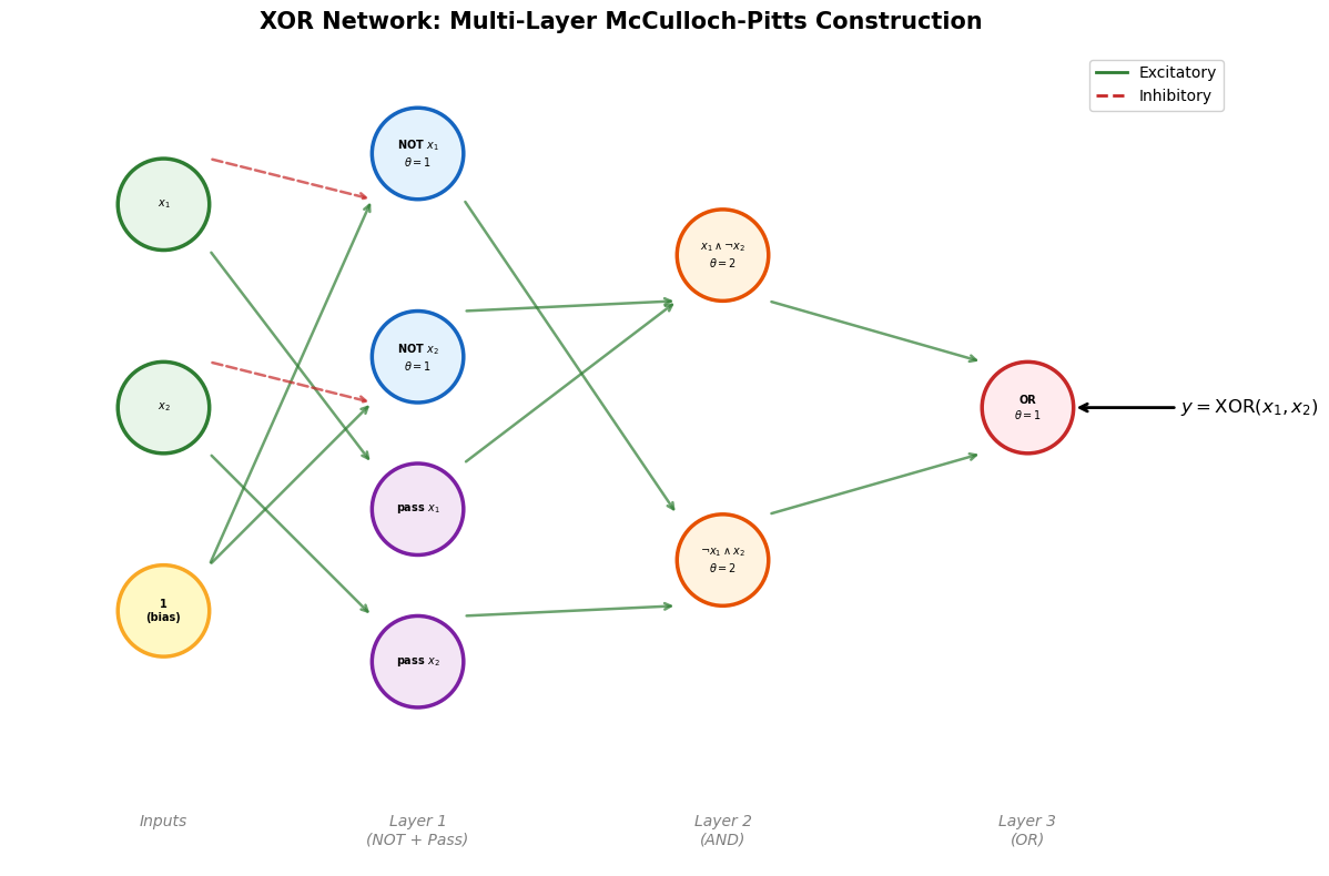
Although a single neuron cannot compute XOR, a network of M-P neurons can. The standard decomposition is:

\[\text{XOR}(x_1, x_2) = (x_1 \wedge \neg x_2) \vee (\neg x_1 \wedge x_2)\]

This requires:

2 NOT neurons (for \(\neg x_1\) and \(\neg x_2\))
2 AND neurons (for \(x_1 \wedge \neg x_2\) and \(\neg x_1 \wedge x_2\))
1 OR neuron (for the final disjunction)

Total: 5 neurons (plus a bias input for the NOT gates).

Tip

The XOR problem is historically one of the most important examples in neural network theory. It demonstrates that depth matters: a single layer cannot do what two layers can. This principle — that deeper networks can compute functions that shallower networks cannot (or can only compute with exponentially more neurons) — is a central theme in modern deep learning theory.

XOR Network Structure:
McCullochPittsNetwork(inputs=3, layers=3)
  Layer 0: ['NOT_x1', 'NOT_x2', 'PASS_x1', 'PASS_x2']
  Layer 1: ['x1_AND_NOTx2', 'NOTx1_AND_x2']
  Layer 2: ['OR_out']

  x1   x2  Expected   Got   Status
--------------------------------
   0    0         0     0     PASS
   0    1         1     1     PASS
   1    0         1     1     PASS
   1    1         0     0     PASS

All tests passed: True
Total neurons used: 5 (2 NOT + 2 AND + 1 OR)

XOR Multi-Layer Network Diagram#

The following visualization shows the complete multi-layer M-P network that computes XOR, illustrating how depth overcomes the limitation of a single neuron.

Show code cell source Hide code cell source

import numpy as np
import matplotlib.pyplot as plt
import matplotlib.patches as mpatches
%matplotlib inline

fig, ax = plt.subplots(figsize=(14, 8))
ax.set_xlim(-1, 11)
ax.set_ylim(-1, 7)
ax.set_aspect('equal')
ax.axis('off')
ax.set_title('XOR Network: Multi-Layer McCulloch-Pitts Construction',
             fontsize=15, fontweight='bold', pad=15)

# Node positions
nodes = {
    'x1': (0.5, 5.5), 'x2': (0.5, 3.5), 'bias': (0.5, 1.5),
    'NOT_x1': (3.0, 6.0), 'NOT_x2': (3.0, 4.0),
    'PASS_x1': (3.0, 2.5), 'PASS_x2': (3.0, 1.0),
    'AND1': (6.0, 5.0), 'AND2': (6.0, 2.0),
    'OR': (9.0, 3.5),
}

node_labels = {
    'x1': '$x_1$', 'x2': '$x_2$', 'bias': '1\n(bias)',
    'NOT_x1': 'NOT $x_1$\n$\\theta=1$', 'NOT_x2': 'NOT $x_2$\n$\\theta=1$',
    'PASS_x1': 'pass $x_1$', 'PASS_x2': 'pass $x_2$',
    'AND1': '$x_1 \\wedge \\neg x_2$\n$\\theta=2$',
    'AND2': '$\\neg x_1 \\wedge x_2$\n$\\theta=2$',
    'OR': 'OR\n$\\theta=1$',
}

node_colors = {
    'x1': ('#E8F5E9', '#2E7D32'), 'x2': ('#E8F5E9', '#2E7D32'),
    'bias': ('#FFF9C4', '#F9A825'),
    'NOT_x1': ('#E3F2FD', '#1565C0'), 'NOT_x2': ('#E3F2FD', '#1565C0'),
    'PASS_x1': ('#F3E5F5', '#7B1FA2'), 'PASS_x2': ('#F3E5F5', '#7B1FA2'),
    'AND1': ('#FFF3E0', '#E65100'), 'AND2': ('#FFF3E0', '#E65100'),
    'OR': ('#FFEBEE', '#C62828'),
}

for name, (x, y) in nodes.items():
    fc, ec = node_colors[name]
    circle = plt.Circle((x, y), 0.45, facecolor=fc, edgecolor=ec, linewidth=2.5, zorder=5)
    ax.add_patch(circle)
    ax.text(x, y, node_labels[name], ha='center', va='center', fontsize=7,
            fontweight='bold', zorder=6)

# Excitatory edges
exc_edges = [
    ('bias', 'NOT_x1'), ('bias', 'NOT_x2'),
    ('x1', 'PASS_x1'), ('x2', 'PASS_x2'),
    ('PASS_x1', 'AND1'), ('NOT_x2', 'AND1'),
    ('NOT_x1', 'AND2'), ('PASS_x2', 'AND2'),
    ('AND1', 'OR'), ('AND2', 'OR'),
]
inh_edges = [('x1', 'NOT_x1'), ('x2', 'NOT_x2')]

for (src, dst) in exc_edges:
    sx, sy = nodes[src]
    dx, dy = nodes[dst]
    ax.annotate('', xy=(dx - 0.45 * np.sign(dx - sx + 0.001), dy - 0.45 * np.sign(dy - sy + 0.001)),
                xytext=(sx + 0.45 * np.sign(dx - sx + 0.001), sy + 0.45 * np.sign(dy - sy + 0.001)),
                arrowprops=dict(arrowstyle='->', color='#2E7D32', lw=1.8, alpha=0.7), zorder=3)

for (src, dst) in inh_edges:
    sx, sy = nodes[src]
    dx, dy = nodes[dst]
    ax.annotate('', xy=(dx - 0.45 * np.sign(dx - sx + 0.001), dy - 0.45 * np.sign(dy - sy + 0.001)),
                xytext=(sx + 0.45 * np.sign(dx - sx + 0.001), sy + 0.45 * np.sign(dy - sy + 0.001)),
                arrowprops=dict(arrowstyle='->', color='#C62828', lw=1.8, linestyle='dashed', alpha=0.7), zorder=3)

# Output arrow
ax.annotate('$y = \\mathrm{XOR}(x_1, x_2)$',
            xy=(9.45, 3.5), xytext=(10.5, 3.5),
            fontsize=12, fontweight='bold', ha='left', va='center',
            arrowprops=dict(arrowstyle='->', color='black', lw=2))

# Layer labels
for lx, label in [(0.5, 'Inputs'), (3.0, 'Layer 1\n(NOT + Pass)'),
                   (6.0, 'Layer 2\n(AND)'), (9.0, 'Layer 3\n(OR)')]:
    ax.text(lx, -0.5, label, ha='center', va='top', fontsize=10,
            fontstyle='italic', color='gray')

legend_elements = [
    plt.Line2D([0], [0], color='#2E7D32', lw=2, label='Excitatory'),
    plt.Line2D([0], [0], color='#C62828', lw=2, linestyle='dashed', label='Inhibitory'),
]
ax.legend(handles=legend_elements, loc='upper right', fontsize=10, framealpha=0.9)

plt.tight_layout()
plt.show()

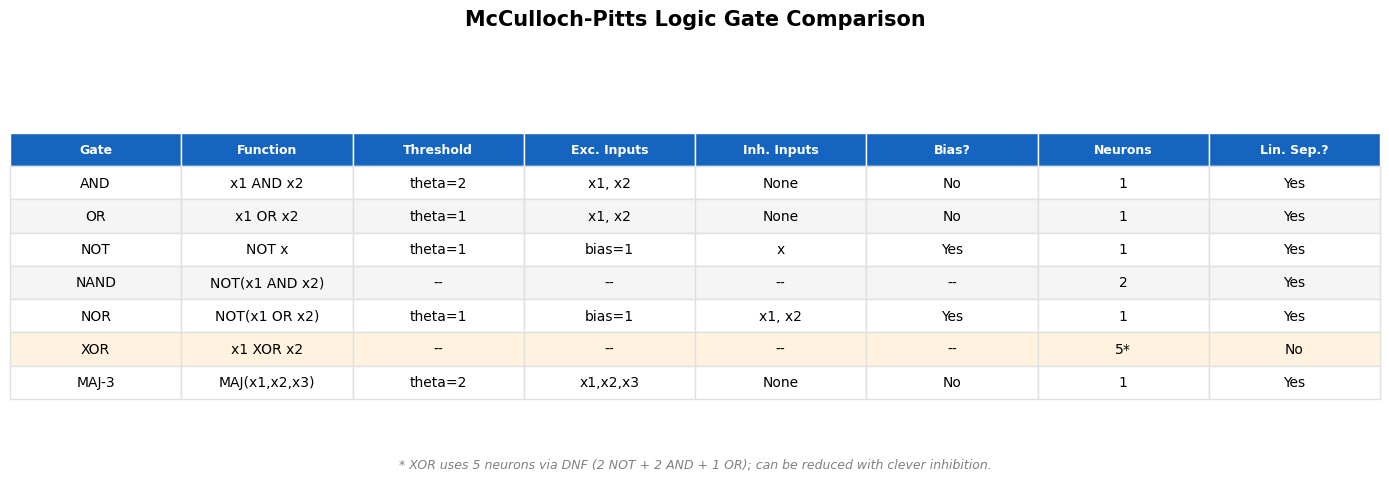
../_images/2fc9938059c126c13a8ba2a816ee4509f12ab9f6f69ac6e60f8a62273e867b30.png

Comparison of Logic Gate Implementations#

The following table summarizes how each common logic gate is implemented using McCulloch-Pitts neurons.

../_images/949d0c18a12153138d9cc9d1785de1d9f3f2008a4799d72326408d5593b5152f.png

Automatically constructed XOR network:
McCullochPittsNetwork(inputs=3, layers=3)
  Layer 0: ['NOT_x0', 'NOT_x1', 'PASS_x0', 'PASS_x1']
  Layer 1: ['MINT_(0, 1)', 'MINT_(1, 0)']
  Layer 2: ['OR_out']

  x1   x2  Expected   Got   Status
--------------------------------
   0    0         0     0     PASS
   0    1         1     1     PASS
   1    0         1     1     PASS
   1    1         0     0     PASS

4. Feedforward vs. Recurrent Networks#

Acyclic (Feedforward) Networks#

Definition (Feedforward Network)

A feedforward M-P network is one whose underlying directed graph is acyclic (has no directed cycles). Signals flow strictly from inputs through layers to outputs, with no feedback. A feedforward M-P network computes a combinational function — its output at time \(t + d\) (where \(d\) is the depth) depends only on the input at time \(t\). It has no memory of previous inputs.

Formally, a feedforward M-P network with \(n\) inputs and \(m\) outputs computes a function:

\[f: \{0,1\}^n \to \{0,1\}^m\]

And we have seen (Theorem I) that every such function is realizable.

Cyclic (Recurrent) Networks#

Definition (Recurrent Network)

A recurrent (cyclic) M-P network is one whose directed graph contains at least one directed cycle. A neuron’s output can, after some number of time steps, feed back into its own input. This creates the possibility of memory — the network’s behavior depends not just on the current input, but on its history.

McCulloch and Pitts recognized this in their original paper. They stated:

Theorem II (McCulloch-Pitts, 1943). Cyclic M-P networks can express temporal propositional expressions that are not bounded in time — i.e., the output can depend on the entire history of inputs.

The simplest example is a latch (also called a flip-flop or set-reset memory).

The Set-Reset Latch#

Consider a neuron \(A\) with threshold \(\theta = 1\) that receives excitatory input from:

An external “set” signal \(S\)
Its own output from the previous time step (feedback)

And an inhibitory input from:

An external “reset” signal \(R\)

The activation rule becomes:

\[A(t+1) = (S(t) \vee A(t)) \wedge \neg R(t)\]

Once \(S\) is pulsed (set to 1 for one time step), the neuron fires and its self-feedback keeps it firing. The only way to turn it off is to pulse \(R\) (reset).

# --- Recurrent M-P Network: SR Latch ---

class RecurrentMPNeuron:
    """A McCulloch-Pitts neuron with recurrent (self-feedback) capability."""

    def __init__(self, threshold, name=None):
        self.threshold = threshold
        self.name = name or f"RMP(theta={threshold})"
        self.state = 0

    def step(self, excitatory_inputs, inhibitory_inputs=None):
        if inhibitory_inputs is not None and any(inhibitory_inputs):
            self.state = 0
        else:
            exc_sum = sum(excitatory_inputs)
            self.state = 1 if exc_sum >= self.threshold else 0
        return self.state

    def reset(self):
        self.state = 0


class SRLatch:
    """Set-Reset latch built from a single recurrent M-P neuron."""

    def __init__(self):
        self.neuron = RecurrentMPNeuron(threshold=1, name='Latch')

    def step(self, set_signal, reset_signal):
        exc = [set_signal, self.neuron.state]
        inh = [reset_signal]
        return self.neuron.step(exc, inh)

    def reset(self):
        self.neuron.reset()

    @property
    def state(self):
        return self.neuron.state


latch = SRLatch()

inputs_sequence = [
    (0, 0), (0, 0), (1, 0), (0, 0), (0, 0), (0, 0),
    (0, 1), (0, 0), (0, 0), (1, 0), (0, 0), (1, 1), (0, 0),
]

print(f"{'t':>3}  {'S':>3}  {'R':>3}  {'Q':>3}  Notes")
print("-" * 40)

history = []
for t, (s, r) in enumerate(inputs_sequence):
    q = latch.step(s, r)
    history.append((t, s, r, q))
    notes = ""
    if s == 1 and r == 0:
        notes = "<-- SET"
    elif s == 0 and r == 1:
        notes = "<-- RESET"
    elif s == 1 and r == 1:
        notes = "<-- S+R (inhibition wins)"
    print(f"{t:>3}  {s:>3}  {r:>3}  {q:>3}  {notes}")

  t    S    R    Q  Notes
----------------------------------------
  0    0    0  
  0    0    0  
  1    0    1  <-- SET
  0    0    1  
  0    0    1  
  0    0    1  
  0    1    0  <-- RESET
  0    0    0  
  0    0    0  
  1    0    1  <-- SET
  0    0    1  
  1    1    0  <-- S+R (inhibition wins)
  0    0    0  

../_images/5eb362bd8f1917cc9e536ad1dbf9c2ffae7e14d667fe447d2331294d4d528443.png

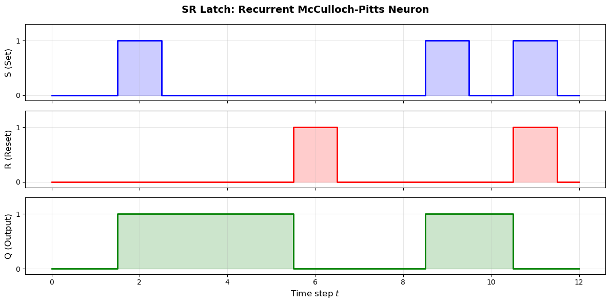
Notice how Q stays latched at 1 after S is pulsed,
and only returns to 0 after R is pulsed. This is memory.

5. Recurrent Network: Extended Example#

Let us build a slightly more complex recurrent example: a toggle flip-flop. This circuit changes state each time a trigger input \(T\) is pulsed.

The behavior we want:

\(Q(t+1) = Q(t) \oplus T(t)\)
When \(T = 0\): hold state (\(Q\) stays the same)
When \(T = 1\): toggle (\(Q\) flips)

This is more complex because XOR itself requires a multi-neuron network, and now we need feedback.

# --- Toggle Flip-Flop using recurrent M-P neurons ---

class ToggleFlipFlop:
    """A toggle flip-flop: Q(t+1) = Q(t) XOR T(t)."""

    def __init__(self):
        self.Q = 0
        self.not_gate = McCullochPittsNeuron(threshold=1, name='NOT')
        self.and_gate = McCullochPittsNeuron(threshold=2, name='AND')
        self.or_gate = McCullochPittsNeuron(threshold=1, name='OR')

    def step(self, T):
        not_T = self.not_gate.activate([1], [T])
        not_Q = self.not_gate.activate([1], [self.Q])
        term1 = self.and_gate.activate([self.Q, not_T])
        term2 = self.and_gate.activate([not_Q, T])
        self.Q = self.or_gate.activate([term1, term2])
        return self.Q

    def reset(self):
        self.Q = 0


tff = ToggleFlipFlop()
trigger_sequence = [0, 0, 1, 0, 0, 1, 1, 0, 1, 0, 0, 1, 0, 0, 1, 1]

print(f"{'t':>3}  {'T':>3}  {'Q':>3}")
print("-" * 15)

tff_history = []
for t, T in enumerate(trigger_sequence):
    q = tff.step(T)
    tff_history.append((t, T, q))
    toggle_mark = " <-- toggle" if T == 1 else ""
    print(f"{t:>3}  {T:>3}  {q:>3}{toggle_mark}")

  t    T    Q
---------------
  0    0
  0    0
  1    1 <-- toggle
  0    1
  0    1
  1    0 <-- toggle
  1    1 <-- toggle
  0    1
  1    0 <-- toggle
  0    0
  0    0
  1    1 <-- toggle
  0    1
  0    1
  1    0 <-- toggle
  1    1 <-- toggle

../_images/a7135e26fe1c1e18260b7382a0a9b8a17cc30efb50320c03b9f739ad293c02c5.png

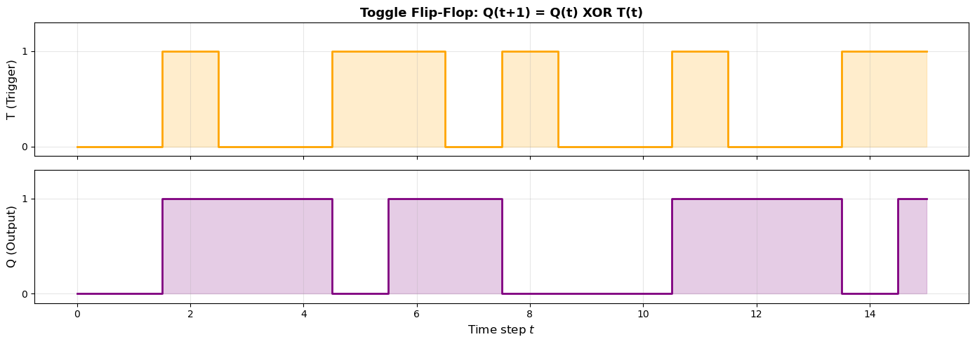
Each time T=1, the output Q toggles (flips between 0 and 1).

6. Turing Equivalence#

Theorem III (McCulloch-Pitts, 1943)#

McCulloch and Pitts claimed, with varying degrees of rigor, that their neural networks with cycles are equivalent in computational power to Turing machines.

Direction 1: M-P Networks can Simulate Finite Automata#

Definition (Finite Automaton)

A finite automaton (FA) is defined by:

A finite set of states \(Q = \{q_0, q_1, \ldots, q_m\}\)
An input alphabet \(\Sigma\)
A transition function \(\delta: Q \times \Sigma \to Q\)
An initial state \(q_0\)
A set of accepting states \(F \subseteq Q\)

Claim. Any finite automaton can be simulated by a cyclic M-P network.

Proof sketch. Encode each state \(q_i\) as a dedicated neuron that is active when the automaton is in that state. The transition function is a Boolean function, implementable by M-P neurons. The recurrence provides state memory. \(\blacksquare\)

Direction 2: Turing Machines can Simulate M-P Networks#

This direction is straightforward: any M-P network with \(n\) neurons can be simulated by a Turing machine that maintains an \(n\)-bit state vector.

The Crucial Nuance#

A finite M-P network has at most \(2^n\) internal states, making it equivalent to a finite automaton, not a full Turing machine. The precise equivalence was clarified by Kleene (1956):

Theorem (Kleene-McCulloch-Pitts)

\[\text{Finite cyclic M-P networks} \equiv \text{Finite automata} \equiv \text{Regular expressions}\]

The class of languages recognized by finite cyclic McCulloch-Pitts networks is precisely the class of regular languages.

Tip

The gap between finite automata and Turing machines is a recurring theme in theoretical computer science. Finite M-P networks compute regular languages; adding an external memory (like a stack) would give context-free languages; adding an unbounded tape gives Turing-completeness. Modern recurrent neural networks (RNNs, LSTMs, Transformers) face analogous questions about their computational power.

7. The Key Limitation: No Learning#

For all their computational power, McCulloch-Pitts networks have a fundamental limitation: there is no mechanism for learning.

Warning

The absence of learning in M-P networks is not just a technical inconvenience — it is a fundamental design limitation. To build an M-P network, you must already know the complete truth table of the function you want to compute. But the whole point of intelligence is dealing with situations you have not seen before. The quest to add learning to neural networks drove the next 40 years of research, from Hebb (1949) through backpropagation (1986).

This means that to build an M-P network for a given task, you must:

Know the desired input-output mapping exactly (the truth table).
Manually design the network (or use the DNF construction).
Accept that the network will never change its behavior.

The recognition of this limitation drove the next major developments:

Donald Hebb (1949): “neurons that fire together, wire together” — the first learning rule.
Frank Rosenblatt (1958): The Perceptron with adjustable weights and a convergence theorem.
Widrow and Hoff (1960): The ADALINE and the delta rule (least mean squares).
Rumelhart, Hinton, and Williams (1986): Backpropagation for multi-layer networks.

The story from McCulloch-Pitts to backpropagation is the story of how the field learned to make neural networks learn.

8. Exercises#

Exercise 2.1: Full Adder#

A full adder takes three 1-bit inputs (\(x_1\), \(x_2\), and carry-in \(c_{\text{in}}\)) and produces:

Sum \(S = x_1 \oplus x_2 \oplus c_{\text{in}}\)
Carry-out \(C_{\text{out}} = (x_1 \wedge x_2) \vee (x_1 \wedge c_{\text{in}}) \vee (x_2 \wedge c_{\text{in}})\)

Build a McCulloch-Pitts network that implements a full adder.

\(x_1\)	\(x_2\)	\(c_{\text{in}}\)	Sum	\(C_{\text{out}}\)
0	0	0	0	0
0	0	1	1	0
0	1	0	1	0
0	1	1	0	1
1	0	0	1	0
1	0	1	0	1
1	1	0	0	1
1	1	1	1	1

Hint

Use the DNF construction for each output separately, or observe that \(C_{\text{out}}\) is the majority function (\(\theta = 2\), three excitatory inputs) and \(S\) is the 3-bit parity function. Parity requires a multi-layer network: chain two XOR computations.

Exercise 2.2: 2-Bit Counter#

Implement a 2-bit binary counter using recurrent M-P neurons. The counter should count up by 1 each time a clock input \(C\) is pulsed: \(00 \to 01 \to 10 \to 11 \to 00 \to \ldots\)

Hint

\(Q_0\) is a toggle flip-flop driven by \(C\). \(Q_1\) is a toggle flip-flop driven by the carry from \(Q_0\) (i.e., \(Q_1\) toggles when \(Q_0\) goes from 1 to 0).

Exercise 2.3: \(n\)-Bit Parity#

The parity function on \(n\) inputs outputs 1 iff the number of 1-inputs is odd:

\[\text{PAR}(x_1, \ldots, x_n) = x_1 \oplus x_2 \oplus \cdots \oplus x_n\]

How many M-P neurons are needed to compute \(n\)-bit parity?

Analysis: The DNF construction uses \(n + 2^{n-1} + 1\) neurons. A tree construction uses \(O(n)\) neurons and \(O(\log n)\) depth.

Hint

For 4-bit parity: compute \(a = x_1 \oplus x_2\) and \(b = x_3 \oplus x_4\) in parallel (each using 5 neurons), then compute \(a \oplus b\) (another 5 neurons). Total: 15 neurons, depth 6. Compare with DNF: \(4 + 8 + 1 = 13\) neurons but only depth 3. There is a tradeoff between number of neurons and depth!

9. Summary#

In this chapter, we have gone from individual McCulloch-Pitts neurons to networks that can compute arbitrary Boolean functions and implement stateful sequential logic.

Key results:#

The DNF construction provides a systematic algorithm to build an M-P network for any Boolean function. The cost is at most \(n + 2^n + 1\) neurons (worst case).
XOR is not computable by a single M-P neuron. This is because XOR is not a threshold function. This is a precursor to Minsky and Papert (1969).
Recurrent (cyclic) M-P networks can implement memory. The SR latch is the simplest example.
Finite cyclic M-P networks are equivalent to finite automata (Kleene-McCulloch-Pitts theorem).
M-P networks have no learning mechanism. Everything is hardwired.

Tip

Looking back at this chapter, notice the pattern: each limitation of a model motivates the next advance. Single neurons cannot compute XOR, so we build networks. Feedforward networks have no memory, so we add cycles. Fixed networks cannot learn, so we introduce adjustable weights. This dialectic of limitation and innovation is the engine that drives the field forward.

The road ahead:#

In the next chapter, we place these results in their historical context, tracing the intellectual lineages from McCulloch and Pitts through the AI winter and up to the backpropagation revolution of 1986.

Chapter 2: Building Logic from Neurons

Contents

Chapter 2: Building Logic from Neurons#

1. Introduction: From Gates to Circuits#

2. The DNF Construction Algorithm#

Theory#

Implementation#

3. XOR: The First Warning Sign#

The Impossibility Result#

Geometric Interpretation#

Building XOR with a Network#

XOR Multi-Layer Network Diagram#

Comparison of Logic Gate Implementations#

4. Feedforward vs. Recurrent Networks#

Acyclic (Feedforward) Networks#

Cyclic (Recurrent) Networks#

The Set-Reset Latch#

5. Recurrent Network: Extended Example#

6. Turing Equivalence#

Theorem III (McCulloch-Pitts, 1943)#

Direction 1: M-P Networks can Simulate Finite Automata#

Direction 2: Turing Machines can Simulate M-P Networks#

The Crucial Nuance#

7. The Key Limitation: No Learning#

8. Exercises#

Exercise 2.1: Full Adder#

Exercise 2.2: 2-Bit Counter#

Exercise 2.3: \(n\)-Bit Parity#

9. Summary#

Key results:#

The road ahead:#