Show code cell source Hide code cell source

import numpy as np
import matplotlib.pyplot as plt

# ── Utility functions ──────────────────────────────────────────────

def softmax(logits):
    shifted = logits - logits.max(axis=1, keepdims=True)
    exp_values = np.exp(shifted)
    return exp_values / exp_values.sum(axis=1, keepdims=True)

def softmax_cross_entropy(logits, targets):
    probabilities = softmax(logits)
    clipped = np.clip(probabilities[np.arange(targets.shape[0]), targets], 1e-12, 1.0)
    loss = -np.log(clipped).mean()
    d_logits = probabilities.copy()
    d_logits[np.arange(targets.shape[0]), targets] -= 1.0
    d_logits /= targets.shape[0]
    return loss, probabilities, d_logits

# ── Layer definitions ──────────────────────────────────────────────

class Conv2D:
    def __init__(self, in_channels, out_channels, kernel_size, seed=42):
        rng = np.random.default_rng(seed)
        fan_in = in_channels * kernel_size * kernel_size
        scale = np.sqrt(2.0 / fan_in)
        self.in_channels = in_channels
        self.out_channels = out_channels
        self.kernel_size = kernel_size
        self.weights = rng.normal(0.0, scale, size=(out_channels, in_channels, kernel_size, kernel_size))
        self.bias = np.zeros(out_channels)
        self.d_weights = np.zeros_like(self.weights)
        self.d_bias = np.zeros_like(self.bias)
        self.last_input = None
    def forward(self, x):
        self.last_input = x
        batch_size, _, height, width = x.shape
        out_h = height - self.kernel_size + 1
        out_w = width - self.kernel_size + 1
        output = np.zeros((batch_size, self.out_channels, out_h, out_w))
        for row in range(out_h):
            for col in range(out_w):
                patch = x[:, :, row:row+self.kernel_size, col:col+self.kernel_size]
                output[:, :, row, col] = np.tensordot(patch, self.weights, axes=([1,2,3],[1,2,3])) + self.bias
        return output
    def backward(self, d_output):
        x = self.last_input
        _, _, out_h, out_w = d_output.shape
        self.d_weights.fill(0.0)
        self.d_bias = d_output.sum(axis=(0, 2, 3))
        d_input = np.zeros_like(x)
        for row in range(out_h):
            for col in range(out_w):
                patch = x[:, :, row:row+self.kernel_size, col:col+self.kernel_size]
                self.d_weights += np.tensordot(d_output[:, :, row, col], patch, axes=([0], [0]))
                d_input[:, :, row:row+self.kernel_size, col:col+self.kernel_size] += np.tensordot(
                    d_output[:, :, row, col], self.weights, axes=([1], [0]))
        return d_input
    def step(self, lr):
        self.weights -= lr * self.d_weights
        self.bias -= lr * self.d_bias
    @property
    def parameter_count(self):
        return int(self.weights.size + self.bias.size)

class ReLU:
    def __init__(self):
        self.last_input = None
    def forward(self, x):
        self.last_input = x
        return np.maximum(0.0, x)
    def backward(self, d_output):
        return d_output * (self.last_input > 0.0)

class MaxPool2D:
    def __init__(self, pool_size=2):
        self.pool_size = pool_size
        self.last_input = None
        self.last_mask = None
    def forward(self, x):
        self.last_input = x
        batch_size, channels, height, width = x.shape
        out_h = height // self.pool_size
        out_w = width // self.pool_size
        output = np.zeros((batch_size, channels, out_h, out_w))
        mask = np.zeros_like(x)
        for row in range(out_h):
            for col in range(out_w):
                rs, cs = row * self.pool_size, col * self.pool_size
                window = x[:, :, rs:rs+self.pool_size, cs:cs+self.pool_size]
                output[:, :, row, col] = window.max(axis=(2, 3))
                flat_idx = window.reshape(batch_size, channels, -1).argmax(axis=2)
                for b in range(batch_size):
                    for c in range(channels):
                        winner = flat_idx[b, c]
                        mask[b, c, rs + winner // self.pool_size, cs + winner % self.pool_size] = 1.0
        self.last_mask = mask
        return output
    def backward(self, d_output):
        d_input = np.zeros_like(self.last_input)
        out_h, out_w = d_output.shape[2], d_output.shape[3]
        for row in range(out_h):
            for col in range(out_w):
                rs, cs = row * self.pool_size, col * self.pool_size
                mask_w = self.last_mask[:, :, rs:rs+self.pool_size, cs:cs+self.pool_size]
                d_input[:, :, rs:rs+self.pool_size, cs:cs+self.pool_size] += (
                    mask_w * d_output[:, :, row, col][:, :, None, None])
        return d_input

class Flatten:
    def __init__(self):
        self.last_shape = None
    def forward(self, x):
        self.last_shape = x.shape
        return x.reshape(x.shape[0], -1)
    def backward(self, d_output):
        return d_output.reshape(self.last_shape)

class Dense:
    def __init__(self, in_features, out_features, seed=42):
        rng = np.random.default_rng(seed)
        scale = np.sqrt(2.0 / in_features)
        self.weights = rng.normal(0.0, scale, size=(in_features, out_features))
        self.bias = np.zeros(out_features)
        self.d_weights = np.zeros_like(self.weights)
        self.d_bias = np.zeros_like(self.bias)
        self.last_input = None
    def forward(self, x):
        self.last_input = x
        return x @ self.weights + self.bias
    def backward(self, d_output):
        self.d_weights = self.last_input.T @ d_output
        self.d_bias = d_output.sum(axis=0)
        return d_output @ self.weights.T
    def step(self, lr):
        self.weights -= lr * self.d_weights
        self.bias -= lr * self.d_bias
    @property
    def parameter_count(self):
        return int(self.weights.size + self.bias.size)

# ── TinyCNN ─────────────────────────────────────────────────────────

class TinyCNN:
    def __init__(self, seed=3, input_size=8, num_classes=3, conv_filters=3):
        rng_seed = seed
        self.conv = Conv2D(1, conv_filters, 3, seed=rng_seed)
        self.relu = ReLU()
        self.pool = MaxPool2D(2)
        self.flatten = Flatten()
        conv_out = input_size - 3 + 1
        pooled = conv_out // 2
        self.dense = Dense(conv_filters * pooled * pooled, num_classes, seed=rng_seed + 1)
        self.num_classes = num_classes
        self.conv_filters = conv_filters

    def forward(self, x):
        return self.dense.forward(self.flatten.forward(self.pool.forward(self.relu.forward(self.conv.forward(x)))))

    def forward_with_trace(self, x):
        """Forward pass returning all intermediate activations."""
        conv_out = self.conv.forward(x)
        relu_out = self.relu.forward(conv_out)
        pool_out = self.pool.forward(relu_out)
        flat_out = self.flatten.forward(pool_out)
        logits = self.dense.forward(flat_out)
        probs = softmax(logits)
        return {
            'input': x,
            'conv': conv_out,
            'relu': relu_out,
            'pool': pool_out,
            'logits': logits,
            'probs': probs,
        }

    def loss_and_grad(self, x, y):
        logits = self.forward(x)
        loss, probs, d_logits = softmax_cross_entropy(logits, y)
        d = self.dense.backward(d_logits)
        d = self.flatten.backward(d)
        d = self.pool.backward(d)
        d = self.relu.backward(d)
        self.conv.backward(d)
        return loss, probs

    def step(self, lr):
        self.conv.step(lr)
        self.dense.step(lr)

    def evaluate(self, x, y):
        logits = self.forward(x)
        loss, _, _ = softmax_cross_entropy(logits, y)
        accuracy = float((logits.argmax(axis=1) == y).mean())
        return loss, accuracy

    def fit(self, x_train, y_train, x_val, y_val, epochs=80, lr=0.12, batch_size=18, seed=11, snapshot_epochs=(0,1,5,15,40,80)):
        rng = np.random.default_rng(seed)
        history = []
        snapshots = []
        def record(ep):
            tl, ta = self.evaluate(x_train, y_train)
            _, va = self.evaluate(x_val, y_val)
            history.append({"epoch": ep, "train_loss": tl, "train_acc": ta, "val_acc": va})
            if ep in snapshot_epochs:
                snapshots.append({"epoch": ep, "kernels": self.conv.weights.copy()})
        record(0)
        for ep in range(1, epochs + 1):
            order = rng.permutation(x_train.shape[0])
            sx, sy = x_train[order], y_train[order]
            for start in range(0, x_train.shape[0], batch_size):
                self.loss_and_grad(sx[start:start+batch_size], sy[start:start+batch_size])
                self.step(lr)
            record(ep)
        return history, snapshots

    @property
    def total_parameters(self):
        return self.conv.parameter_count + self.dense.parameter_count

# ── TinyMLP ─────────────────────────────────────────────────────────

class TinyMLP:
    def __init__(self, seed=5, input_size=8, hidden_size=18, num_classes=3):
        rng = np.random.default_rng(seed)
        flat_size = input_size * input_size
        self.flatten = Flatten()
        self.hidden = Dense(flat_size, hidden_size, seed=seed)
        self.relu = ReLU()
        self.output = Dense(hidden_size, num_classes, seed=seed + 1)
        self.num_classes = num_classes

    def forward(self, x):
        return self.output.forward(self.relu.forward(self.hidden.forward(self.flatten.forward(x))))

    def loss_and_grad(self, x, y):
        logits = self.forward(x)
        loss, probs, d_logits = softmax_cross_entropy(logits, y)
        d = self.output.backward(d_logits)
        d = self.relu.backward(d)
        d = self.hidden.backward(d)
        self.flatten.backward(d)
        return loss, probs

    def step(self, lr):
        self.hidden.step(lr)
        self.output.step(lr)

    def evaluate(self, x, y):
        logits = self.forward(x)
        loss, _, _ = softmax_cross_entropy(logits, y)
        accuracy = float((logits.argmax(axis=1) == y).mean())
        return loss, accuracy

    def fit(self, x_train, y_train, x_val, y_val, epochs=80, lr=0.12, batch_size=18, seed=13):
        rng = np.random.default_rng(seed)
        history = []
        def record(ep):
            tl, ta = self.evaluate(x_train, y_train)
            _, va = self.evaluate(x_val, y_val)
            history.append({"epoch": ep, "train_loss": tl, "train_acc": ta, "val_acc": va})
        record(0)
        for ep in range(1, epochs + 1):
            order = rng.permutation(x_train.shape[0])
            sx, sy = x_train[order], y_train[order]
            for start in range(0, x_train.shape[0], batch_size):
                self.loss_and_grad(sx[start:start+batch_size], sy[start:start+batch_size])
                self.step(lr)
            record(ep)
        return history

    @property
    def total_parameters(self):
        return self.hidden.parameter_count + self.output.parameter_count

# ── Dataset ──────────────────────────────────────────────────────────

CLASS_NAMES = ("vertical", "horizontal", "diagonal")
DOT_CLASS_NAMES = ("vertical", "horizontal", "diagonal", "dot")

def _pattern_for_class(name, size):
    pattern = np.zeros((size, size))
    c = size // 2
    if name == "vertical": pattern[:, c-1:c+1] = 1.0
    elif name == "horizontal": pattern[c-1:c+1, :] = 1.0
    elif name == "diagonal":
        np.fill_diagonal(pattern, 1.0)
        pattern += 0.35 * np.eye(size, k=1) + 0.35 * np.eye(size, k=-1)
    elif name == "dot": pattern[c-1:c+1, c-1:c+1] = 1.0
    return np.clip(pattern, 0.0, 1.0)

def make_dataset(train_per_class=60, val_per_class=30, size=8, seed=7, class_names=CLASS_NAMES):
    rng = np.random.default_rng(seed)
    total = train_per_class + val_per_class
    patterns = [_pattern_for_class(n, size) for n in class_names]
    all_x, all_y = [], []
    for label, pat in enumerate(patterns):
        for _ in range(total):
            img = pat.copy()
            sy, sx = rng.integers(-1, 2, size=2)
            shifted = np.zeros_like(img)
            src_ys = max(0, -sy); src_ye = size - max(0, sy)
            src_xs = max(0, -sx); src_xe = size - max(0, sx)
            dst_ys = max(0, sy); dst_xs = max(0, sx)
            shifted[dst_ys:dst_ys+(src_ye-src_ys), dst_xs:dst_xs+(src_xe-src_xs)] = img[src_ys:src_ye, src_xs:src_xe]
            canvas = shifted * rng.uniform(0.85, 1.15)
            canvas += rng.normal(0, 0.12, (size, size))
            all_x.append(np.clip(canvas, 0, 1))
            all_y.append(label)
    x = np.array(all_x)[:, None, :, :]
    y = np.array(all_y, dtype=np.int64)
    rng2 = np.random.default_rng(seed + 99)
    xt, yt, xv, yv = [], [], [], []
    for label in range(len(class_names)):
        idx = np.where(y == label)[0]
        order = rng2.permutation(len(idx))
        idx = idx[order]
        xt.append(x[idx[:train_per_class]]); yt.append(y[idx[:train_per_class]])
        xv.append(x[idx[train_per_class:]]); yv.append(y[idx[train_per_class:]])
    x_train = np.concatenate(xt); y_train = np.concatenate(yt)
    x_val = np.concatenate(xv); y_val = np.concatenate(yv)
    order_t = rng2.permutation(len(x_train)); order_v = rng2.permutation(len(x_val))
    return x_train[order_t], y_train[order_t], x_val[order_v], y_val[order_v]

# ── Plot styling ─────────────────────────────────────────────────────

CREAM = '#fdf6ec'
CNN_BLUE = '#22577a'
MLP_RED = '#bc4749'
GREEN_LIGHT = '#55a630'
GREEN_DARK = '#2b9348'

def style_ax(ax, title=None, xlabel=None, ylabel=None):
    ax.set_facecolor(CREAM)
    if title: ax.set_title(title, fontsize=13, fontweight='bold', pad=8)
    if xlabel: ax.set_xlabel(xlabel, fontsize=11)
    if ylabel: ax.set_ylabel(ylabel, fontsize=11)
    ax.spines['top'].set_visible(False)
    ax.spines['right'].set_visible(False)
    ax.grid(True, alpha=0.3, linestyle='--')

print('Infrastructure loaded: Conv2D, ReLU, MaxPool2D, Flatten, Dense, TinyCNN, TinyMLP, make_dataset')

Infrastructure loaded: Conv2D, ReLU, MaxPool2D, Flatten, Dense, TinyCNN, TinyMLP, make_dataset

Chapter 25: CNN Experiments and Analysis

In the previous chapter we built a convolutional neural network from scratch and watched it learn to classify simple 8\(\times\)8 patterns. Now we turn to the experimental side: How does the CNN compare to a plain fully-connected network? How sensitive is the MLP baseline to its hidden-layer width? What happens when we add a fourth pattern class? And what, exactly, do the learned convolutional filters look like?

This chapter is heavy on visualization and analysis. Every figure is generated from our pure-NumPy implementations; no external deep-learning library is used.

25.1 CNN vs MLP Baseline

Our first experiment is the most natural one: train both architectures on the same 3-class data and compare them.

The TinyCNN uses 3 convolutional filters of size \(3\times 3\) followed by ReLU, \(2\times 2\) max-pooling, flattening, and a dense output layer. The TinyMLP flattens the image directly and passes it through a hidden layer of 18 units with ReLU, then a dense output layer.

We train both for 80 epochs with learning rate \(\eta = 0.12\) and batch size 18.

Show code cell source Hide code cell source

# Train CNN and MLP on the 3-class dataset
x_train, y_train, x_val, y_val = make_dataset()

cnn = TinyCNN(seed=3)
cnn_history, cnn_snapshots = cnn.fit(x_train, y_train, x_val, y_val)

mlp = TinyMLP(seed=5)
mlp_history = mlp.fit(x_train, y_train, x_val, y_val)

# Two-panel figure: training curves and parameter counts
fig, (ax1, ax2) = plt.subplots(1, 2, figsize=(11, 4.2))
fig.patch.set_facecolor(CREAM)

# Left: validation accuracy curves
cnn_epochs = [h['epoch'] for h in cnn_history]
cnn_val = [h['val_acc'] for h in cnn_history]
mlp_epochs = [h['epoch'] for h in mlp_history]
mlp_val = [h['val_acc'] for h in mlp_history]

ax1.plot(cnn_epochs, cnn_val, color=CNN_BLUE, linewidth=2.2, label=f'TinyCNN ({cnn.total_parameters} params)')
ax1.plot(mlp_epochs, mlp_val, color=MLP_RED, linewidth=2.2, linestyle='--', label=f'TinyMLP ({mlp.total_parameters} params)')
ax1.axhline(1.0, color='grey', linewidth=0.8, linestyle=':')
ax1.set_ylim(0.0, 1.08)
style_ax(ax1, title='Validation Accuracy', xlabel='Epoch', ylabel='Accuracy')
ax1.legend(fontsize=10, loc='lower right', framealpha=0.9)

# Right: parameter count bar chart
models = ['TinyCNN', 'TinyMLP']
params = [cnn.total_parameters, mlp.total_parameters]
colors = [CNN_BLUE, MLP_RED]
bars = ax2.bar(models, params, color=colors, width=0.5, edgecolor='white', linewidth=1.5)
for bar, p in zip(bars, params):
    ax2.text(bar.get_x() + bar.get_width()/2, bar.get_height() + 20,
             f'{p:,}', ha='center', va='bottom', fontsize=12, fontweight='bold')
style_ax(ax2, title='Parameter Count', ylabel='Number of Parameters')
ax2.set_ylim(0, max(params) * 1.25)

fig.suptitle('CNN vs MLP on 3-Class Pattern Recognition', fontsize=14, fontweight='bold', y=1.02)
plt.tight_layout()
plt.show()

# Print final results
cnn_final = cnn_history[-1]
mlp_final = mlp_history[-1]
print(f'CNN  final accuracy: train={cnn_final["train_acc"]:.3f}, val={cnn_final["val_acc"]:.3f}  ({cnn.total_parameters} parameters)')
print(f'MLP  final accuracy: train={mlp_final["train_acc"]:.3f}, val={mlp_final["val_acc"]:.3f}  ({mlp.total_parameters} parameters)')
print(f'Parameter ratio:     MLP / CNN = {mlp.total_parameters / cnn.total_parameters:.1f}x')

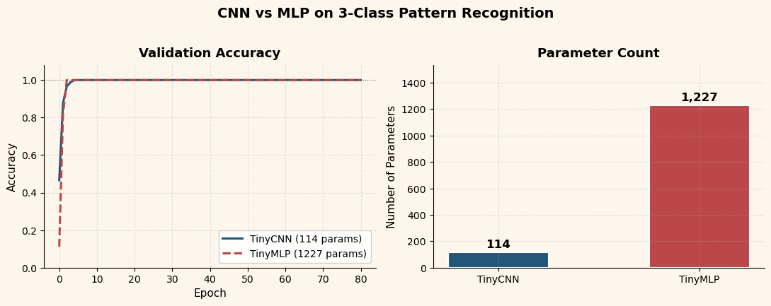
CNN  final accuracy: train=1.000, val=1.000  (114 parameters)
MLP  final accuracy: train=1.000, val=1.000  (1227 parameters)
Parameter ratio:     MLP / CNN = 10.8x

Key Observation

On this toy task, both architectures achieve excellent accuracy. The CNN advantage is not in final accuracy but in parameter efficiency and interpretability: the CNN uses roughly 10\(\times\) fewer parameters, and its learned filters have a clear visual meaning (as we will see in Section 25.5).

The MLP must learn separate weights for every pixel position, while the CNN re-uses the same small \(3\times 3\) kernel across the entire image. This weight sharing is the source of the parameter savings.

25.2 Hidden-Width Capacity Sweep

The TinyMLP with 18 hidden units has more than enough capacity for our 3-class task. But what happens if we shrink the hidden layer? At what point does the MLP fail, and how does its stability change?

We sweep over hidden-layer widths \(h \in \{1, 2, 3, 4, 6, 10, 18\}\) and train 5 random seeds per width. For each width we report the mean, minimum, and maximum validation accuracy across seeds.

Show code cell source Hide code cell source

# Capacity sweep: MLP hidden-width from 1 to 18
widths = [1, 2, 3, 4, 6, 10, 18]
seeds = list(range(5))
sweep_results = {}

for w in widths:
    accs = []
    for s in seeds:
        model = TinyMLP(seed=s, hidden_size=w)
        hist = model.fit(x_train, y_train, x_val, y_val, seed=s + 100)
        accs.append(hist[-1]['val_acc'])
    sweep_results[w] = {'mean': np.mean(accs), 'min': np.min(accs),
                        'max': np.max(accs), 'all': accs}

# CNN reference (single value)
cnn_ref_acc = cnn_history[-1]['val_acc']

# Band plot
fig, ax = plt.subplots(figsize=(8, 4.5))
fig.patch.set_facecolor(CREAM)

means = [sweep_results[w]['mean'] for w in widths]
mins = [sweep_results[w]['min'] for w in widths]
maxs = [sweep_results[w]['max'] for w in widths]

ax.fill_between(widths, mins, maxs, color=MLP_RED, alpha=0.18, label='MLP min/max range')
ax.plot(widths, means, color=MLP_RED, linewidth=2.2, marker='o', markersize=6, label='MLP mean accuracy')
ax.axhline(cnn_ref_acc, color=CNN_BLUE, linewidth=2.0, linestyle='--',
           label=f'CNN ({cnn.total_parameters} params)')

# Mark the "first stable" width
ax.axvline(4, color=GREEN_DARK, linewidth=1.2, linestyle=':', alpha=0.7)
ax.annotate('first stable\nwidth', xy=(4, 0.55), fontsize=9, color=GREEN_DARK,
            ha='center', style='italic')

style_ax(ax, title='MLP Validation Accuracy vs Hidden-Layer Width',
         xlabel='Hidden units', ylabel='Validation accuracy')
ax.set_xticks(widths)
ax.set_ylim(0.2, 1.08)
ax.legend(fontsize=10, loc='lower right', framealpha=0.9)
plt.tight_layout()
plt.show()

# Print table
print(f'{"Width":>6} {"Mean":>8} {"Min":>8} {"Max":>8}')
print('-' * 34)
for w in widths:
    r = sweep_results[w]
    print(f'{w:>6} {r["mean"]:>8.3f} {r["min"]:>8.3f} {r["max"]:>8.3f}')

 Width     Mean      Min      Max
----------------------------------
     1    0.864    0.333    1.000
     2    0.989    0.956    1.000
     3    1.000    1.000    1.000
     4    1.000    1.000    1.000
     6    1.000    1.000    1.000
    10    1.000    1.000    1.000
    18    1.000    1.000    1.000

The sweep reveals a clear pattern:

• Width 1 consistently fails: a single hidden unit cannot separate three classes (it can only create two half-spaces in the feature space).

• Width 2–3 is unstable: some seeds converge, others do not. The network is operating at the edge of its representational capacity.

• Width 4 is the first width where all five seeds achieve high accuracy. This aligns with theory: \(k\) classes require at least \(k+1\) hidden units in the worst case for non-degenerate decision boundaries.

• Width 10–18 gives uniformly high accuracy with no seed sensitivity.

Capacity vs Inductive Bias

The MLP needs at least 4 hidden units to reliably solve a 3-class problem on 8\(\times\)8 images. The CNN, by contrast, solves the same problem with only 3 convolutional filters plus a small output head. The difference is inductive bias: the CNN’s built-in assumptions (local connectivity, weight sharing, translation equivariance) make the hypothesis space much smaller, so fewer parameters suffice.

25.3 Adding a Fourth Class

Our original dataset has three pattern classes: vertical, horizontal, and diagonal bars. What happens when we add a fourth class – a centered dot pattern?

For the CNN, we keep the same 3 convolutional filters and simply grow the output layer from 3 to 4 units. For the MLP, we keep hidden_size=18 and also grow the output layer.

The central question: Does the CNN need more filters?

Show code cell source Hide code cell source

# Four-class dataset
x4_train, y4_train, x4_val, y4_val = make_dataset(class_names=DOT_CLASS_NAMES)

# Train CNN (3 filters, 4 classes)
cnn4 = TinyCNN(seed=3, num_classes=4, conv_filters=3)
cnn4_history, _ = cnn4.fit(x4_train, y4_train, x4_val, y4_val)

# Train MLP (hidden=18, 4 classes)
mlp4 = TinyMLP(seed=5, hidden_size=18, num_classes=4)
mlp4_history = mlp4.fit(x4_train, y4_train, x4_val, y4_val)

# Two-panel comparison: 3-class vs 4-class
fig, (ax1, ax2) = plt.subplots(1, 2, figsize=(11, 4.2))
fig.patch.set_facecolor(CREAM)

# Left: 3-class results
ax1.plot(cnn_epochs, cnn_val, color=CNN_BLUE, linewidth=2.2, label='CNN (3 filters)')
ax1.plot(mlp_epochs, mlp_val, color=MLP_RED, linewidth=2.2, linestyle='--', label='MLP (h=18)')
ax1.axhline(1.0, color='grey', linewidth=0.8, linestyle=':')
ax1.set_ylim(0.0, 1.08)
style_ax(ax1, title='3-Class Task', xlabel='Epoch', ylabel='Validation Accuracy')
ax1.legend(fontsize=9, loc='lower right', framealpha=0.9)

# Right: 4-class results
cnn4_epochs = [h['epoch'] for h in cnn4_history]
cnn4_val = [h['val_acc'] for h in cnn4_history]
mlp4_epochs = [h['epoch'] for h in mlp4_history]
mlp4_val = [h['val_acc'] for h in mlp4_history]

ax2.plot(cnn4_epochs, cnn4_val, color=CNN_BLUE, linewidth=2.2, label=f'CNN (3 filters, {cnn4.total_parameters} params)')
ax2.plot(mlp4_epochs, mlp4_val, color=MLP_RED, linewidth=2.2, linestyle='--', label=f'MLP (h=18, {mlp4.total_parameters} params)')
ax2.axhline(1.0, color='grey', linewidth=0.8, linestyle=':')
ax2.set_ylim(0.0, 1.08)
style_ax(ax2, title='4-Class Task (+ dot)', xlabel='Epoch', ylabel='Validation Accuracy')
ax2.legend(fontsize=9, loc='lower right', framealpha=0.9)

fig.suptitle('Scaling from 3 to 4 Classes', fontsize=14, fontweight='bold', y=1.02)
plt.tight_layout()
plt.show()

print(f'4-class CNN:  val_acc = {cnn4_history[-1]["val_acc"]:.3f}  ({cnn4.total_parameters} params, 3 filters)')
print(f'4-class MLP:  val_acc = {mlp4_history[-1]["val_acc"]:.3f}  ({mlp4.total_parameters} params, h=18)')

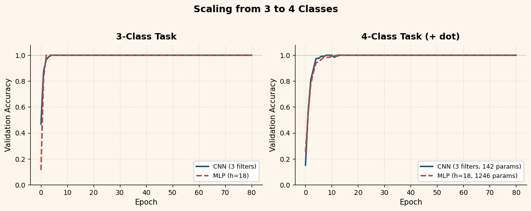
4-class CNN:  val_acc = 1.000  (142 params, 3 filters)
4-class MLP:  val_acc = 1.000  (1246 params, h=18)

The answer is no – the CNN does not need more convolutional filters to handle the fourth class. The convolutional layers act as a general-purpose feature extractor: they detect oriented edges and local intensity patterns regardless of how many classes the output head must distinguish. Adding a fourth class only requires one more output neuron in the dense layer, adding just \(3 \times 3 + 1 = 10\) parameters (one weight per pooled feature map location, plus one bias).

This separation between the feature extractor and the classifier head is one of the most important architectural ideas in deep learning. It is the basis for transfer learning: pre-train the convolutional layers on a large dataset, then replace only the output head for a new task.

25.4 Inference Trace

To build intuition for what happens inside the CNN, we take a single input image and trace it through every stage of the pipeline:

\[ \text{Input} \;\xrightarrow{\text{Conv}}\; \text{Feature maps} \;\xrightarrow{\text{ReLU}}\; \text{Activations} \;\xrightarrow{\text{MaxPool}}\; \text{Pooled maps} \;\xrightarrow{\text{Dense + Softmax}}\; \text{Class probabilities} \]

We use the CNN trained on the 3-class data (from Section 25.1) and pass a single vertical-bar sample through it.

Show code cell source Hide code cell source

# Pick a vertical-bar sample from validation set
vert_idx = np.where(y_val == 0)[0][0]
sample = x_val[vert_idx:vert_idx+1]  # shape (1, 1, 8, 8)

# Trace through the trained CNN
trace = cnn.forward_with_trace(sample)

n_filters = cnn.conv_filters
fig, axes = plt.subplots(5, n_filters, figsize=(9, 12),
                         gridspec_kw={'height_ratios': [1.2, 1.0, 1.0, 0.8, 1.0]})
fig.patch.set_facecolor(CREAM)

# Row 0: Input image (span all filter columns)
for j in range(n_filters):
    axes[0, j].set_visible(False)
ax_input = fig.add_axes([0.35, 0.82, 0.3, 0.14])  # manual positioning
ax_input.imshow(sample[0, 0], cmap='gray', vmin=0, vmax=1, aspect='equal')
ax_input.set_title('Input (8x8)', fontsize=11, fontweight='bold')
ax_input.set_xticks([]); ax_input.set_yticks([])
ax_input.patch.set_facecolor(CREAM)

# Row 1: Conv output (3 feature maps, 6x6)
for j in range(n_filters):
    im = axes[1, j].imshow(trace['conv'][0, j], cmap='RdBu_r', aspect='equal')
    axes[1, j].set_title(f'Conv filter {j}', fontsize=9)
    axes[1, j].set_xticks([]); axes[1, j].set_yticks([])
    axes[1, j].patch.set_facecolor(CREAM)
fig.text(0.02, 0.68, 'Conv\nOutput', fontsize=10, fontweight='bold', va='center', ha='center')

# Row 2: ReLU output
for j in range(n_filters):
    axes[2, j].imshow(trace['relu'][0, j], cmap='Oranges', aspect='equal', vmin=0)
    axes[2, j].set_title(f'ReLU {j}', fontsize=9)
    axes[2, j].set_xticks([]); axes[2, j].set_yticks([])
    axes[2, j].patch.set_facecolor(CREAM)
fig.text(0.02, 0.52, 'ReLU\nOutput', fontsize=10, fontweight='bold', va='center', ha='center')

# Row 3: Pooled output (3x3)
for j in range(n_filters):
    axes[3, j].imshow(trace['pool'][0, j], cmap='Oranges', aspect='equal', vmin=0)
    axes[3, j].set_title(f'Pool {j}', fontsize=9)
    axes[3, j].set_xticks([]); axes[3, j].set_yticks([])
    axes[3, j].patch.set_facecolor(CREAM)
fig.text(0.02, 0.36, 'MaxPool\nOutput', fontsize=10, fontweight='bold', va='center', ha='center')

# Row 4: Softmax bar chart (span all columns)
for j in range(n_filters):
    axes[4, j].set_visible(False)
ax_bar = fig.add_axes([0.2, 0.05, 0.6, 0.15])
probs = trace['probs'][0]
bar_colors = [CNN_BLUE if i == 0 else '#aaaaaa' for i in range(len(probs))]
bars = ax_bar.barh(CLASS_NAMES[:len(probs)], probs, color=bar_colors, edgecolor='white', height=0.5)
for bar, p in zip(bars, probs):
    ax_bar.text(bar.get_width() + 0.02, bar.get_y() + bar.get_height()/2,
               f'{p:.3f}', va='center', fontsize=10, fontweight='bold')
ax_bar.set_xlim(0, 1.15)
ax_bar.set_title('Softmax Probabilities', fontsize=11, fontweight='bold')
ax_bar.set_facecolor(CREAM)
ax_bar.spines['top'].set_visible(False)
ax_bar.spines['right'].set_visible(False)

fig.suptitle('Inference Trace: Vertical Bar through TinyCNN', fontsize=14,
             fontweight='bold', y=0.99)
plt.show()

Reading the trace from top to bottom:

1. Input: the 8\(\times\)8 grayscale image shows a vertical bar (two bright columns in the center).

2. Conv output: each of the 3 learned filters responds differently to the input. Some filters produce strong positive responses where the bar is, others are more muted.

3. ReLU output: negative activations are zeroed out. Only the regions where a filter truly “fires” remain.

4. MaxPool output: the 6\(\times\)6 feature maps are reduced to 3\(\times\)3 by taking the maximum in each 2\(\times\)2 window. This provides a small degree of translation invariance.

5. Softmax output: the dense layer combines the 27 pooled features into class logits, and softmax converts them to probabilities. The network correctly assigns the highest probability to “vertical”.

25.5 What the Filters Learn

Perhaps the most compelling aspect of convolutional networks is that the learned filters are interpretable. Each \(3\times 3\) kernel is a tiny template that the network slides across the image, computing a local similarity score at each position.

Let us visualize the three learned kernels from the trained CNN and see what patterns they detect.

Show code cell source Hide code cell source

# Visualize learned kernels
kernels = cnn.conv.weights  # shape (3, 1, 3, 3)

fig, axes = plt.subplots(1, 3, figsize=(9, 3.5))
fig.patch.set_facecolor(CREAM)

vmax = np.abs(kernels).max()
for i in range(3):
    k = kernels[i, 0]  # shape (3, 3)
    im = axes[i].imshow(k, cmap='RdBu_r', vmin=-vmax, vmax=vmax, aspect='equal')
    axes[i].set_title(f'Filter {i}', fontsize=12, fontweight='bold')
    axes[i].set_xticks(range(3)); axes[i].set_yticks(range(3))
    axes[i].patch.set_facecolor(CREAM)
    # Annotate each weight value
    for r in range(3):
        for c in range(3):
            val = k[r, c]
            color = 'white' if abs(val) > vmax * 0.6 else 'black'
            axes[i].text(c, r, f'{val:.2f}', ha='center', va='center',
                        fontsize=9, fontweight='bold', color=color)

fig.colorbar(im, ax=axes, fraction=0.02, pad=0.04, label='Weight value')
fig.suptitle('Learned Convolutional Filters (3x3)', fontsize=14, fontweight='bold')
fig.subplots_adjust(top=0.85, bottom=0.05, wspace=0.3)
plt.show()

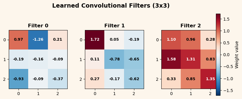
The trained filters typically show clear oriented-edge structure:

• One filter develops a vertical gradient (strong positive weights in a column, negative or near-zero elsewhere) – it responds to vertical edges.

• Another develops a horizontal gradient – it responds to horizontal edges.

• The third often captures diagonal or more complex patterns.

These are exactly the features needed to distinguish our three pattern classes. The network has discovered, through gradient descent alone, that oriented edge detection is the right strategy.

Connection to Neuroscience

In 1959, David Hubel and Torsten Wiesel discovered that neurons in the cat’s primary visual cortex respond selectively to oriented edges at specific positions in the visual field. They called these simple cells. The filters learned by our CNN bear a striking resemblance to simple-cell receptive fields: small, spatially localized, and orientation-selective. This parallel between biological vision and artificial convolutional networks is not accidental – Kunihiko Fukushima explicitly cited Hubel and Wiesel’s work when he designed the Neocognitron (1980), the direct ancestor of modern CNNs.

25.6 Scaling Up: From 8x8 to Real Images

Our TinyCNN operates on 8\(\times\)8 grayscale images with 3 filters and a single convolutional layer. Real-world convolutional networks follow the same architectural pattern – Conv \(\to\) ReLU \(\to\) Pool \(\to\) Dense – but at vastly larger scale. Let us trace the historical progression:

Network	Year	Input Size	Layers	Parameters	Key Innovation
LeNet-5 (LeCun)	1998	32\(\times\)32	7	60K	Proven on MNIST digits
AlexNet (Krizhevsky)	2012	227\(\times\)227	8	60M	GPU training, dropout, ReLU
VGG-16 (Simonyan)	2014	224\(\times\)224	16	138M	Uniform 3\(\times\)3 filters throughout
ResNet-50 (He)	2015	224\(\times\)224	50	25M	Skip connections, batch normalization

Several patterns emerge:

Depth increases. LeNet-5 has 2 convolutional layers; ResNet-50 has 49. Deeper networks can learn hierarchical features: early layers detect edges, middle layers detect textures and parts, and deep layers detect whole objects.

Filter counts grow with depth. A typical pattern is 64 filters in the first layer, 128 in the second, 256 in the third, and so on. As spatial resolution decreases (through pooling), the number of feature channels increases.

The core operation is unchanged. Every network in the table above uses the same cross-correlation operation we implemented in Conv2D.forward. The mathematical foundations from our toy example carry over directly.

From MNIST to ImageNet

LeNet-5 was designed for the MNIST handwritten digit dataset (10 classes, 60,000 training images of 28\(\times\)28 pixels). AlexNet was the first CNN to win the ImageNet Large Scale Visual Recognition Challenge (1,000 classes, 1.2 million training images of roughly 256\(\times\)256 pixels). The jump from MNIST to ImageNet required not just bigger networks, but also GPU computing, data augmentation, and regularization techniques like dropout – topics that go beyond our classical foundations but build directly on the principles we have studied.

Exercises

Exercise 25.1. Add a fifth class to the dataset (for example, a “cross” pattern that combines vertical and horizontal bars). Train the CNN with 3 filters. Does it still achieve high accuracy? At what point (how many classes) do 3 filters become insufficient?

Exercise 25.2. Modify Conv2D to support a \(2\times 2\) kernel instead of \(3\times 3\). Train on the 3-class data and compare the learned filters. Are \(2\times 2\) kernels expressive enough to distinguish the patterns? What about \(5\times 5\)? (Note: a \(5\times 5\) kernel on an \(8\times 8\) input produces only a \(4\times 4\) feature map, and after \(2\times 2\) pooling you get \(2\times 2\). This still works but leaves very little spatial information.)

Exercise 25.3. Implement strided convolution by adding a stride parameter to Conv2D. With stride=2, the kernel moves two pixels at a time instead of one, reducing the output size without needing a separate pooling layer. Train a CNN that uses Conv2D with stride=2 and no MaxPool2D. Compare the results.

Exercise 25.4. Implement a simple dropout layer that randomly zeroes out activations during training (with probability \(p = 0.3\)) and scales the remaining activations by \(\frac{1}{1-p}\). During evaluation, dropout should be a no-op. Insert it between the flatten and dense layers of TinyCNN. Does it help on this toy task? (Hint: dropout is most useful when the model is overfitting, which our small CNN does not.)

Exercise 25.5. Run the capacity sweep from Section 25.2 but for the CNN instead: vary the number of convolutional filters from 1 to 8. How does the CNN’s accuracy change? Is the CNN more or less sensitive to this hyperparameter than the MLP is to its hidden width?