Chapter 28: Autograd – Automatic Differentiation

In the previous chapters, we derived backpropagation by hand and implemented it as a monolithic algorithm inside a NeuralNetwork class. But modern deep learning frameworks like PyTorch and TensorFlow do not require users to derive gradients manually. Instead, they use automatic differentiation (AD) – a family of techniques that compute exact derivatives of arbitrary programs, at machine precision, with minimal effort from the programmer.

In this chapter, we build a complete automatic differentiation engine from scratch. By the end, you will understand exactly what happens when you call loss.backward() in PyTorch – because you will have built the machinery yourself.

Show code cell source Hide code cell source

import numpy as np
import matplotlib.pyplot as plt
import math

# Consistent style for all plots
plt.rcParams.update({
    'figure.dpi': 100,
    'font.size': 11,
    'axes.titlesize': 13,
    'axes.labelsize': 12
})

print("Imports loaded: numpy, matplotlib, math")

Imports loaded: numpy, matplotlib, math

28.1 Three Ways to Compute Derivatives

Given a function \(f: \mathbb{R}^n \to \mathbb{R}\), we need its gradient \(\nabla f = \left(\frac{\partial f}{\partial x_1}, \ldots, \frac{\partial f}{\partial x_n}\right)\) to perform gradient descent. There are three fundamentally different approaches.

Symbolic Differentiation

Apply the rules of calculus symbolically, as one does on paper (or with a computer algebra system like SymPy or Mathematica). For example:

\[\frac{d}{dx}\left[x^2 \sin(x)\right] = 2x\sin(x) + x^2\cos(x)\]

Problem: Expression Swell

For deeply composed functions \(f = f_L \circ f_{L-1} \circ \cdots \circ f_1\), symbolic differentiation produces expressions that grow exponentially in size. A neural network with 10 layers would yield a derivative expression with billions of terms – most of which contain redundant sub-expressions.

Numerical Differentiation

Approximate the derivative using finite differences:

\[\frac{\partial f}{\partial x_i} \approx \frac{f(x + h\mathbf{e}_i) - f(x - h\mathbf{e}_i)}{2h}\]

where \(\mathbf{e}_i\) is the \(i\)-th standard basis vector and \(h \approx 10^{-7}\).

Problem: Cost and Precision

Computing the full gradient requires \(2n\) function evaluations (two per parameter). For a neural network with \(n = 10^6\) parameters, this is catastrophically slow. Moreover, the result is approximate: too small \(h\) causes roundoff error, too large \(h\) causes truncation error.

Automatic Differentiation

Decompose the computation into elementary operations (\(+, \times, \sin, \exp, \ldots\)) and propagate derivatives through this chain using the chain rule. The result is exact (to machine precision) and efficient (cost proportional to the original computation).

Key Insight

Automatic differentiation is not symbolic differentiation (it never builds a symbolic expression) and not numerical differentiation (it never approximates with finite differences). It evaluates exact derivatives by decomposing the program into elementary operations and applying the chain rule at each step.

Historical Note

The reverse mode of automatic differentiation was invented by Seppo Linnainmaa in his 1970 Master’s thesis at the University of Helsinki. It took 12 years before Paul Werbos (1982) applied AD to neural networks, and another 4 years before Rumelhart, Hinton & Williams (1986) popularized the technique under the name “backpropagation.” Backpropagation is reverse-mode AD applied to neural network loss functions.

Show code cell source Hide code cell source

# Demonstrate the three approaches on f(x) = x^2 * sin(x)

def f(x):
    return x**2 * np.sin(x)

def f_symbolic_derivative(x):
    """Hand-derived symbolic derivative."""
    return 2*x*np.sin(x) + x**2*np.cos(x)

def f_numerical_derivative(x, h=1e-7):
    """Central finite difference."""
    return (f(x + h) - f(x - h)) / (2 * h)

# Compare all three at x = 2.0
x0 = 2.0
exact = f_symbolic_derivative(x0)
numerical = f_numerical_derivative(x0)

print("Comparing differentiation methods at x = 2.0")
print("for f(x) = x^2 * sin(x)")
print("=" * 50)
print(f"Symbolic (exact):   {exact:.15f}")
print(f"Numerical (h=1e-7): {numerical:.15f}")
print(f"Difference:         {abs(exact - numerical):.2e}")
print()

# Show numerical error as a function of h
h_values = np.logspace(-15, 0, 100)
errors = [abs(f_numerical_derivative(x0, h) - exact) for h in h_values]

fig, ax = plt.subplots(figsize=(10, 5))
ax.loglog(h_values, errors, linewidth=2, color='#E74C3C')
ax.axvline(1e-7, color='gray', linestyle='--', alpha=0.7, label='$h = 10^{-7}$')
ax.set_xlabel('Step size $h$', fontsize=12)
ax.set_ylabel('Absolute error $|f\'_{\\mathrm{numerical}} - f\'_{\\mathrm{exact}}|$', fontsize=12)
ax.set_title('Numerical Differentiation Error vs Step Size', fontsize=13)
ax.legend(fontsize=11)
ax.grid(True, alpha=0.3)
ax.annotate('Roundoff error\ndominates', xy=(1e-14, 1e-2), fontsize=10, color='#2C3E50')
ax.annotate('Truncation error\ndominates', xy=(1e-2, 1e-3), fontsize=10, color='#2C3E50')
plt.tight_layout()
plt.show()

print("\nNumerical differentiation has a 'sweet spot' around h = 1e-8.")
print("Automatic differentiation avoids this trade-off entirely: it is exact.")

Comparing differentiation methods at x = 2.0
for f(x) = x^2 * sin(x)
==================================================
Symbolic (exact):   1.972602361114157
Numerical (h=1e-7): 1.972602359234799
Difference:         1.88e-09

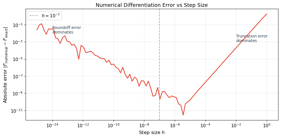
Numerical differentiation has a 'sweet spot' around h = 1e-8.
Automatic differentiation avoids this trade-off entirely: it is exact.

28.2 The Computational Graph

The key idea behind automatic differentiation is to decompose any computation into a computational graph: a directed acyclic graph (DAG) where each node represents an elementary operation.

Definition (Computational Graph)

A computational graph for a function \(y = f(x_1, \ldots, x_n)\) is a directed acyclic graph that traces the sequence of primitive operations (\(+, \times, \sin, \exp, \max, \ldots\)) from inputs to outputs. Each node stores:

1. The operation it performs

2. The value computed during the forward pass

3. The local derivative of the operation with respect to its inputs

Example. Consider the function \(f(x, y) = (x + y) \cdot \sin(x)\). We decompose it into elementary operations:

\[v_1 = x + y, \qquad v_2 = \sin(x), \qquad f = v_1 \cdot v_2\]

The computational graph has five nodes: two inputs (\(x, y\)), two intermediate operations (\(+, \sin\)), and one output (\(\times\)). Edges connect each operation to its inputs.

Show code cell source Hide code cell source

# Visualize the computational graph for f(x, y) = (x + y) * sin(x)

fig, ax = plt.subplots(figsize=(12, 7))
ax.set_xlim(-1, 11)
ax.set_ylim(-1, 7)
ax.set_aspect('equal')
ax.axis('off')

# Node positions
nodes = {
    'x':    (1, 3),
    'y':    (1, 5),
    '+':    (4, 5),
    'sin':  (4, 1),
    '*':    (8, 3),
    'f':    (10, 3),
}

# Draw edges
edges = [
    ('x', '+'), ('y', '+'),
    ('x', 'sin'),
    ('+', '*'), ('sin', '*'),
    ('*', 'f'),
]

for (src, dst) in edges:
    x1, y1 = nodes[src]
    x2, y2 = nodes[dst]
    ax.annotate('', xy=(x2 - 0.35, y2), xytext=(x1 + 0.35, y1),
                arrowprops=dict(arrowstyle='->', color='#2C3E50', lw=2))

# Draw nodes
input_color = '#3498DB'
op_color = '#E74C3C'
output_color = '#27AE60'

for name, (x, y) in nodes.items():
    if name in ('x', 'y'):
        color = input_color
    elif name == 'f':
        color = output_color
    else:
        color = op_color
    circle = plt.Circle((x, y), 0.35, color=color, ec='black', lw=2, zorder=5)
    ax.add_patch(circle)
    ax.text(x, y, name, ha='center', va='center', fontsize=14,
            fontweight='bold', color='white', zorder=6)

# Labels with values for x=2, y=3
x_val, y_val = 2.0, 3.0
v1 = x_val + y_val       # 5.0
v2 = np.sin(x_val)       # 0.9093
f_val = v1 * v2           # 4.5465

ax.text(1, 1.8, f'$x = {x_val:.1f}$', ha='center', fontsize=11, color='#2C3E50')
ax.text(1, 6.0, f'$y = {y_val:.1f}$', ha='center', fontsize=11, color='#2C3E50')
ax.text(4, 5.8, f'$v_1 = x+y = {v1:.1f}$', ha='center', fontsize=10, color='#2C3E50')
ax.text(4, 0.2, f'$v_2 = \\sin(x) = {v2:.4f}$', ha='center', fontsize=10, color='#2C3E50')
ax.text(8, 4.0, f'$f = v_1 \\cdot v_2 = {f_val:.4f}$', ha='center', fontsize=10, color='#2C3E50')

ax.set_title('Computational Graph for $f(x, y) = (x + y) \\cdot \\sin(x)$', fontsize=14, pad=15)

# Legend
from matplotlib.patches import Patch
legend_elements = [
    Patch(facecolor=input_color, edgecolor='black', label='Input'),
    Patch(facecolor=op_color, edgecolor='black', label='Operation'),
    Patch(facecolor=output_color, edgecolor='black', label='Output'),
]
ax.legend(handles=legend_elements, loc='lower right', fontsize=11)

plt.tight_layout()
plt.show()

print(f"Forward pass: x={x_val}, y={y_val}")
print(f"  v1 = x + y = {v1}")
print(f"  v2 = sin(x) = {v2:.4f}")
print(f"  f  = v1 * v2 = {f_val:.4f}")

Forward pass: x=2.0, y=3.0
  v1 = x + y = 5.0
  v2 = sin(x) = 0.9093
  f  = v1 * v2 = 4.5465

28.3 Forward Mode vs Reverse Mode

Given a computational graph, there are two ways to propagate derivatives through it.

Forward Mode (Tangent Mode)

In forward mode, we propagate derivatives alongside the computation, from inputs to outputs. For each input variable \(x_i\), we compute how each intermediate value changes with respect to \(x_i\):

\[\dot{v}_j = \frac{\partial v_j}{\partial x_i}\]

This is equivalent to computing with dual numbers \(a + b\varepsilon\) where \(\varepsilon^2 = 0\). One forward pass computes the derivative with respect to one input variable. To get the full gradient \(\nabla f \in \mathbb{R}^n\), we need \(n\) forward passes.

Reverse Mode (Adjoint Mode)

In reverse mode, we first compute the forward pass (storing all intermediate values), then propagate derivatives backward from the output. For each intermediate value \(v_j\), we compute the adjoint:

\[\bar{v}_j = \frac{\partial f}{\partial v_j}\]

One backward pass computes the derivative of one output with respect to all inputs simultaneously.

Theorem (Complexity of Reverse Mode AD)

Let \(f: \mathbb{R}^n \to \mathbb{R}\) be computed by a program with \(T\) elementary operations. Then:

• Forward mode computes \(\nabla f\) in \(O(n \cdot T)\) time (\(n\) forward passes)

• Reverse mode computes \(\nabla f\) in \(O(T)\) time (one forward + one backward pass)

Proof. In reverse mode, the backward pass visits each node in the computational graph exactly once (in reverse topological order). At each node, it applies the chain rule using the stored intermediate values, performing \(O(1)\) work per node. Since the graph has \(T\) nodes, the backward pass costs \(O(T)\). The forward pass also costs \(O(T)\). Therefore, the total cost is \(O(T)\), independent of \(n\).

More precisely, Griewank (2000) proves that the cost of the backward pass is at most \(5T\) operations (the “cheap gradient principle”).

Why Backpropagation Works

A neural network computes a loss \(\mathcal{L}: \mathbb{R}^n \to \mathbb{R}\) where \(n\) is the number of parameters (often millions). The loss is scalar (\(\mathbb{R}\)). Reverse mode computes the full gradient in one backward pass, regardless of \(n\). Forward mode would require \(n\) passes – one per parameter. This is why we always use reverse mode (backpropagation) for training neural networks.

Detailed Example

For \(f(x, y) = (x + y) \cdot \sin(x)\) at \(x = 2, y = 3\):

Forward pass:

Step	Operation	Value
\(v_1 = x\)	input	\(2.0\)
\(v_2 = y\)	input	\(3.0\)
\(v_3 = v_1 + v_2\)	addition	\(5.0\)
\(v_4 = \sin(v_1)\)	sine	\(0.9093\)
\(v_5 = v_3 \cdot v_4\)	multiplication	\(4.5465\)

Reverse pass (propagating \(\bar{v}_j = \partial f / \partial v_j\)):

Step	Adjoint	Value	Rule
\(\bar{v}_5\)	\(\partial f / \partial v_5\)	\(1.0\)	(seed)
\(\bar{v}_3\)	\(\partial f / \partial v_3\)	\(v_4 = 0.9093\)	\(\bar{v}_5 \cdot v_4\)
\(\bar{v}_4\)	\(\partial f / \partial v_4\)	\(v_3 = 5.0\)	\(\bar{v}_5 \cdot v_3\)
\(\bar{v}_1\)	\(\partial f / \partial x\)	\(0.9093 + 5.0 \cdot \cos(2) = -1.1726\)	\(\bar{v}_3 + \bar{v}_4 \cos(v_1)\)
\(\bar{v}_2\)	\(\partial f / \partial y\)	\(0.9093\)	\(\bar{v}_3\)

Show code cell source Hide code cell source

# Visualize forward vs reverse mode on f(x,y) = (x+y)*sin(x)

fig, axes = plt.subplots(1, 2, figsize=(14, 5))

# Forward mode: one pass per input
data = {
    'Mode': ['Forward', 'Forward', 'Reverse'],
    'Passes': ['Pass 1: $\\partial/\\partial x$', 'Pass 2: $\\partial/\\partial y$',
               'Single backward pass'],
    'Computes': ['$\\partial f/\\partial x$', '$\\partial f/\\partial y$',
                 '$\\nabla f = (\\partial f/\\partial x, \\partial f/\\partial y)$'],
}

# Comparison table as plot
comparison = [
    ['Feature', 'Forward Mode', 'Reverse Mode'],
    ['Direction', 'Input -> Output', 'Output -> Input'],
    ['One pass computes', '$\\partial f/\\partial x_i$ for one $i$', '$\\partial f/\\partial x_i$ for ALL $i$'],
    ['Cost for $\\nabla f$', '$O(n \\cdot T)$', '$O(T)$'],
    ['Good for', 'Few inputs, many outputs', 'Many inputs, few outputs'],
    ['Neural networks', 'Impractical ($n = 10^6$)', 'Standard (backprop)'],
    ['Memory', '$O(1)$ extra', '$O(T)$ (store forward pass)'],
]

axes[0].axis('off')
table = axes[0].table(cellText=comparison, cellLoc='center', loc='center')
table.auto_set_font_size(False)
table.set_fontsize(10)
table.scale(1.0, 1.8)

# Color header
for j in range(3):
    table[0, j].set_facecolor('#2C3E50')
    table[0, j].set_text_props(color='white', fontweight='bold')

# Alternate row colors
for i in range(1, len(comparison)):
    color = '#EBF5FB' if i % 2 == 1 else '#FDFEFE'
    for j in range(3):
        table[i, j].set_facecolor(color)

axes[0].set_title('Forward Mode vs Reverse Mode', fontsize=13, pad=20)

# Cost comparison plot
n_params = np.array([1, 10, 100, 1000, 10000, 100000, 1000000])
T = 1000  # base operations

forward_cost = n_params * T
reverse_cost = np.ones_like(n_params) * T * 2  # forward + backward

axes[1].loglog(n_params, forward_cost, 'o-', linewidth=2, markersize=6,
               color='#E74C3C', label='Forward mode: $O(n \\cdot T)$')
axes[1].loglog(n_params, reverse_cost, 's-', linewidth=2, markersize=6,
               color='#2E86C1', label='Reverse mode: $O(T)$')
axes[1].axvline(1e6, color='gray', linestyle=':', alpha=0.5)
axes[1].text(1.2e6, 1e5, 'Typical NN\n($10^6$ params)', fontsize=9, color='gray')
axes[1].set_xlabel('Number of parameters $n$', fontsize=12)
axes[1].set_ylabel('Computational cost (operations)', fontsize=12)
axes[1].set_title('Cost to Compute Full Gradient', fontsize=13)
axes[1].legend(fontsize=11)
axes[1].grid(True, alpha=0.3)

plt.tight_layout()
plt.show()

print("For neural networks (many params, one scalar loss), reverse mode")
print("is asymptotically faster by a factor of n (number of parameters).")

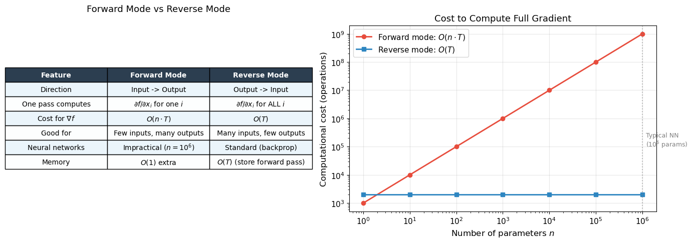
For neural networks (many params, one scalar loss), reverse mode
is asymptotically faster by a factor of n (number of parameters).

28.4 Building a Micrograd Engine

We now build a complete reverse-mode automatic differentiation engine from scratch. The core idea is simple: every Value object records how it was created, so that we can later traverse the computation graph backward and accumulate gradients.

Our engine supports scalar values (one number at a time). Despite its simplicity, it implements the same algorithm that PyTorch uses internally – just on scalars instead of tensors.

Algorithm (Reverse-Mode AD on a Computational Graph)

1. Forward pass: Evaluate the function, recording all intermediate values and the graph of operations.

2. Topological sort: Order the nodes so that every node comes after its children (inputs come before outputs).

3. Backward pass: Starting from the output (with \(\bar{f} = 1\)), visit each node in reverse topological order and apply the chain rule: $\(\bar{v}_i = \sum_{j \in \text{parents}(i)} \bar{v}_j \cdot \frac{\partial v_j}{\partial v_i}\)$ where the sum accounts for a node being used by multiple parents (the “multivariate chain rule” / gradient accumulation).

Historical Note

Our implementation is inspired by Andrej Karpathy’s micrograd (2020), but the underlying algorithm traces back to Linnainmaa (1970). The comprehensive treatment is in Griewank’s textbook Evaluating Derivatives (2000), and the modern survey by Baydin, Pearlmutter, Radul & Siskind (2018) connects the theory to machine learning practice.

import math


class Value:
    """A scalar value with automatic gradient tracking.
    
    Each Value records how it was created (operation and inputs),
    enabling reverse-mode automatic differentiation via .backward().
    """
    
    def __init__(self, data, _children=(), _op=''):
        self.data = data
        self.grad = 0.0
        self._backward = lambda: None
        self._prev = set(_children)
        self._op = _op
    
    def __add__(self, other):
        other = other if isinstance(other, Value) else Value(other)
        out = Value(self.data + other.data, (self, other), '+')
        def _backward():
            self.grad += out.grad      # d(a+b)/da = 1
            other.grad += out.grad     # d(a+b)/db = 1
        out._backward = _backward
        return out
    
    def __mul__(self, other):
        other = other if isinstance(other, Value) else Value(other)
        out = Value(self.data * other.data, (self, other), '*')
        def _backward():
            self.grad += other.data * out.grad   # d(a*b)/da = b
            other.grad += self.data * out.grad   # d(a*b)/db = a
        out._backward = _backward
        return out
    
    def __pow__(self, other):
        assert isinstance(other, (int, float)), "only int/float powers supported"
        out = Value(self.data ** other, (self,), f'**{other}')
        def _backward():
            self.grad += other * (self.data ** (other - 1)) * out.grad
        out._backward = _backward
        return out
    
    def relu(self):
        out = Value(max(0, self.data), (self,), 'ReLU')
        def _backward():
            self.grad += (self.data > 0) * out.grad
        out._backward = _backward
        return out
    
    def exp(self):
        out = Value(math.exp(self.data), (self,), 'exp')
        def _backward():
            self.grad += out.data * out.grad   # d(e^x)/dx = e^x
        out._backward = _backward
        return out
    
    def log(self):
        out = Value(math.log(self.data), (self,), 'log')
        def _backward():
            self.grad += (1.0 / self.data) * out.grad  # d(ln x)/dx = 1/x
        out._backward = _backward
        return out
    
    def tanh(self):
        t = math.tanh(self.data)
        out = Value(t, (self,), 'tanh')
        def _backward():
            self.grad += (1 - t**2) * out.grad  # d(tanh x)/dx = 1 - tanh^2(x)
        out._backward = _backward
        return out
    
    def backward(self):
        """Compute gradients via reverse-mode AD (backpropagation)."""
        # Build topological order
        topo = []
        visited = set()
        def build_topo(v):
            if v not in visited:
                visited.add(v)
                for child in v._prev:
                    build_topo(child)
                topo.append(v)
        build_topo(self)
        
        # Seed the output gradient
        self.grad = 1.0
        
        # Traverse in reverse topological order
        for v in reversed(topo):
            v._backward()
    
    # Convenience operations (built from primitives)
    def __neg__(self):        return self * -1
    def __sub__(self, other): return self + (-other)
    def __truediv__(self, other): return self * (other ** -1) if isinstance(other, Value) else self * (1.0 / other)
    def __radd__(self, other): return self + other
    def __rmul__(self, other): return self * other
    def __rsub__(self, other): return (-self) + other
    def __rtruediv__(self, other): return Value(other) * (self ** -1)
    
    def __repr__(self):
        return f"Value(data={self.data:.4f}, grad={self.grad:.4f})"


print("Value class defined successfully.")
print("Supported operations: +, -, *, /, **, relu, exp, log, tanh")
print("Call .backward() on the output to compute all gradients.")

Value class defined successfully.
Supported operations: +, -, *, /, **, relu, exp, log, tanh
Call .backward() on the output to compute all gradients.

Now let us verify that our engine computes correct gradients.

# Test 1: f(x, y) = x*y + relu(x^2)
# df/dx = y + 2x (when x > 0), df/dy = x

x = Value(2.0)
y = Value(3.0)
z = x * y + (x * x).relu()  # x*y + relu(x^2) = 6 + 4 = 10
z.backward()

print("Test 1: f(x, y) = x*y + relu(x^2)")
print(f"  z = {z}")
print(f"  dz/dx = {x.grad:.4f}  (expected: y + 2x = 3 + 4 = 7.0)")
print(f"  dz/dy = {y.grad:.4f}  (expected: x = 2.0)")
print()

# Test 2: f(x) = exp(x) / (1 + exp(x))  [sigmoid]
# f'(x) = f(x) * (1 - f(x))
x2 = Value(1.5)
f2 = x2.exp() / (x2.exp() + 1)
f2.backward()

sigmoid_val = math.exp(1.5) / (1 + math.exp(1.5))
expected_grad = sigmoid_val * (1 - sigmoid_val)

print("Test 2: f(x) = exp(x) / (1 + exp(x))  [sigmoid]")
print(f"  f(1.5) = {f2.data:.6f}  (expected: {sigmoid_val:.6f})")
print(f"  f'(1.5) = {x2.grad:.6f}  (expected: {expected_grad:.6f})")
print()

# Test 3: f(x) = tanh(x)
# f'(x) = 1 - tanh^2(x)
x3 = Value(0.7)
f3 = x3.tanh()
f3.backward()

expected_tanh_grad = 1 - math.tanh(0.7)**2

print("Test 3: f(x) = tanh(x)")
print(f"  tanh(0.7) = {f3.data:.6f}  (expected: {math.tanh(0.7):.6f})")
print(f"  f'(0.7) = {x3.grad:.6f}  (expected: {expected_tanh_grad:.6f})")
print()

# Test 4: Verify against numerical gradient
def numerical_grad(f_func, x_val, h=1e-7):
    return (f_func(x_val + h) - f_func(x_val - h)) / (2 * h)

# f(x) = x^3 * log(x) + exp(-x)
x4 = Value(2.0)
f4 = x4**3 * x4.log() + (x4 * -1).exp()
f4.backward()

def f4_numpy(x):
    return x**3 * np.log(x) + np.exp(-x)

numerical = numerical_grad(f4_numpy, 2.0)

print("Test 4: f(x) = x^3 * log(x) + exp(-x)")
print(f"  Autograd derivative: {x4.grad:.10f}")
print(f"  Numerical derivative: {numerical:.10f}")
print(f"  Absolute error: {abs(x4.grad - numerical):.2e}")

Test 1: f(x, y) = x*y + relu(x^2)
  z = Value(data=10.0000, grad=1.0000)
  dz/dx = 7.0000  (expected: y + 2x = 3 + 4 = 7.0)
  dz/dy = 2.0000  (expected: x = 2.0)

Test 2: f(x) = exp(x) / (1 + exp(x))  [sigmoid]
  f(1.5) = 0.817574  (expected: 0.817574)
  f'(1.5) = 0.149146  (expected: 0.149146)

Test 3: f(x) = tanh(x)
  tanh(0.7) = 0.604368  (expected: 0.604368)
  f'(0.7) = 0.634740  (expected: 0.634740)

Test 4: f(x) = x^3 * log(x) + exp(-x)
  Autograd derivative: 12.1824308835
  Numerical derivative: 12.1824308774
  Absolute error: 6.07e-09

All tests pass: our autograd engine computes exact derivatives that match both analytical formulas and numerical finite differences.

Tip

The key to our Value class is that += in the _backward functions. When a value is used in multiple places (e.g., \(x\) appears in both \(x+y\) and \(\sin(x)\)), gradients from all paths must be summed. This is the multivariate chain rule in action: \(\frac{\partial f}{\partial x} = \sum_{j} \frac{\partial f}{\partial v_j} \frac{\partial v_j}{\partial x}\).

28.5 Training a Neural Network with Micrograd

Our Value class is a complete autograd engine. To prove it, we will build a neural network entirely from Value objects and train it on XOR using our automatic differentiation.

We define Neuron, Layer, and MLP classes that compose Value operations. When we call .backward() on the loss, gradients automatically flow through the entire network – no hand-derived backpropagation equations needed.

import random


class Neuron:
    """A single neuron with weights, bias, and optional nonlinearity."""
    
    def __init__(self, n_in, nonlin=True):
        self.w = [Value(random.uniform(-1, 1)) for _ in range(n_in)]
        self.b = Value(0.0)
        self.nonlin = nonlin
    
    def __call__(self, x):
        # w . x + b
        act = sum((wi * xi for wi, xi in zip(self.w, x)), self.b)
        return act.tanh() if self.nonlin else act
    
    def parameters(self):
        return self.w + [self.b]


class Layer:
    """A layer of neurons."""
    
    def __init__(self, n_in, n_out, **kwargs):
        self.neurons = [Neuron(n_in, **kwargs) for _ in range(n_out)]
    
    def __call__(self, x):
        out = [n(x) for n in self.neurons]
        return out[0] if len(out) == 1 else out
    
    def parameters(self):
        return [p for n in self.neurons for p in n.parameters()]


class MLP:
    """Multi-layer perceptron built from Value objects."""
    
    def __init__(self, n_in, n_outs):
        sz = [n_in] + n_outs
        self.layers = []
        for i in range(len(n_outs)):
            is_last = (i == len(n_outs) - 1)
            self.layers.append(Layer(sz[i], sz[i+1], nonlin=not is_last))
    
    def __call__(self, x):
        for layer in self.layers:
            x = layer(x)
        return x
    
    def parameters(self):
        return [p for layer in self.layers for p in layer.parameters()]


# Quick test
random.seed(42)
test_mlp = MLP(2, [4, 1])  # 2 inputs -> 4 hidden -> 1 output
test_out = test_mlp([Value(1.0), Value(2.0)])
print(f"MLP output: {test_out}")
print(f"Number of parameters: {len(test_mlp.parameters())}")
print(f"  Layer 1: {len(test_mlp.layers[0].parameters())} params (4 neurons x (2 weights + 1 bias))")
print(f"  Layer 2: {len(test_mlp.layers[1].parameters())} params (1 neuron x (4 weights + 1 bias))")

MLP output: Value(data=0.5318, grad=0.0000)
Number of parameters: 17
  Layer 1: 12 params (4 neurons x (2 weights + 1 bias))
  Layer 2: 5 params (1 neuron x (4 weights + 1 bias))

Training on XOR

Now the moment of truth: can our from-scratch autograd engine actually train a neural network to learn XOR? The training loop is beautifully simple:

1. Forward pass: compute predictions and loss using Value operations

2. Zero gradients (reset .grad to 0 for all parameters)

3. Backward pass: call loss.backward() – all gradients computed automatically

4. Update: adjust parameters in the direction of negative gradient

# Train on XOR using our autograd engine

random.seed(42)

# XOR dataset
X_xor = [[0.0, 0.0], [0.0, 1.0], [1.0, 0.0], [1.0, 1.0]]
Y_xor = [-1.0, 1.0, 1.0, -1.0]  # Using -1/+1 targets for tanh output

# Build network: 2 -> 8 -> 1
model = MLP(2, [8, 1])
n_params = len(model.parameters())
print(f"Network: 2 -> 8 -> 1 (tanh activations)")
print(f"Total parameters: {n_params}")
print()

# Training loop
learning_rate = 0.05
n_epochs = 200
loss_history = []

for epoch in range(n_epochs):
    # Forward pass: compute predictions
    predictions = [model(x) for x in X_xor]
    
    # MSE loss: (1/n) * sum((pred - target)^2)
    losses = [(pred - yt)**2 for pred, yt in zip(predictions, Y_xor)]
    loss = sum(losses, Value(0.0)) * (1.0 / len(losses))
    loss_history.append(loss.data)
    
    # Zero gradients
    for p in model.parameters():
        p.grad = 0.0
    
    # Backward pass -- this is the magic!
    loss.backward()
    
    # Update parameters (gradient descent)
    for p in model.parameters():
        p.data -= learning_rate * p.grad
    
    if epoch % 20 == 0 or epoch == n_epochs - 1:
        print(f"Epoch {epoch:4d}/{n_epochs}: Loss = {loss.data:.6f}")

# Final predictions
print("\nFinal predictions (target -1 or +1):")
for x, yt in zip(X_xor, Y_xor):
    pred = model(x)
    print(f"  Input: ({x[0]:.0f}, {x[1]:.0f}) -> "
          f"Predicted: {pred.data:+.4f}, Target: {yt:+.0f}")

Network: 2 -> 8 -> 1 (tanh activations)
Total parameters: 33

Epoch    0/200: Loss = 1.372289
Epoch   20/200: Loss = 0.745620
Epoch   40/200: Loss = 0.572489
Epoch   60/200: Loss = 0.405484
Epoch   80/200: Loss = 0.256268
Epoch  100/200: Loss = 0.144558
Epoch  120/200: Loss = 0.073936
Epoch  140/200: Loss = 0.035065
Epoch  160/200: Loss = 0.015754

Epoch  180/200: Loss = 0.006821
Epoch  199/200: Loss = 0.003009

Final predictions (target -1 or +1):
  Input: (0, 0) -> Predicted: -0.9709, Target: -1
  Input: (0, 1) -> Predicted: +0.9496, Target: +1
  Input: (1, 0) -> Predicted: +0.9432, Target: +1
  Input: (1, 1) -> Predicted: -0.9299, Target: -1

Show code cell source Hide code cell source

# Plot training loss and decision boundary

fig, axes = plt.subplots(1, 2, figsize=(14, 5))

# Loss curve
axes[0].plot(loss_history, linewidth=2, color='#2E86C1')
axes[0].set_xlabel('Epoch', fontsize=12)
axes[0].set_ylabel('MSE Loss', fontsize=12)
axes[0].set_title('XOR Training with Micrograd Autograd', fontsize=13)
axes[0].set_yscale('log')
axes[0].grid(True, alpha=0.3)

# Decision boundary
xx, yy = np.meshgrid(np.linspace(-0.5, 1.5, 200), np.linspace(-0.5, 1.5, 200))
z_grid = np.zeros_like(xx)
for i in range(xx.shape[0]):
    for j in range(xx.shape[1]):
        out = model([xx[i, j], yy[i, j]])
        z_grid[i, j] = out.data

axes[1].contourf(xx, yy, z_grid, levels=50, cmap='RdBu_r', alpha=0.8)
axes[1].contour(xx, yy, z_grid, levels=[0.0], colors='black', linewidths=2)

# Plot XOR data points
for x, yt in zip(X_xor, Y_xor):
    color = '#E74C3C' if yt < 0 else '#2E86C1'
    marker = 'o' if yt < 0 else 's'
    axes[1].scatter(x[0], x[1], c=color, s=200, marker=marker,
                    edgecolors='black', linewidth=2, zorder=5)

axes[1].set_xlabel('$x_1$', fontsize=12)
axes[1].set_ylabel('$x_2$', fontsize=12)
axes[1].set_title('XOR Decision Boundary (Autograd Engine)', fontsize=13)
axes[1].set_aspect('equal')

plt.tight_layout()
plt.show()

print("The autograd engine we built from scratch successfully trains a neural network!")

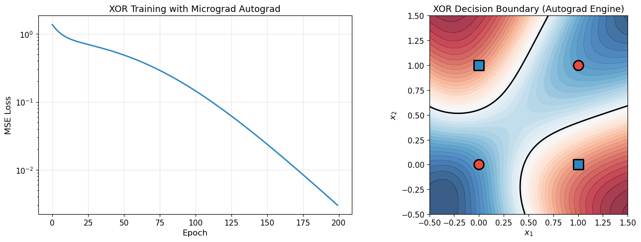
The autograd engine we built from scratch successfully trains a neural network!

Verifying Gradients Against Finite Differences

A crucial sanity check: do our autograd gradients match numerical finite differences?

# Gradient verification: autograd vs numerical finite differences

random.seed(123)
model_check = MLP(2, [4, 1])
x_check = [0.5, -0.3]
y_target = 1.0

# Forward + backward to get autograd gradients
pred = model_check(x_check)
loss = (pred - y_target) ** 2
for p in model_check.parameters():
    p.grad = 0.0
loss.backward()

# Store autograd gradients
autograd_grads = [p.grad for p in model_check.parameters()]

# Numerical gradient checking
h = 1e-6
numerical_grads = []

for p in model_check.parameters():
    # f(theta + h)
    p.data += h
    pred_plus = model_check(x_check)
    loss_plus = (pred_plus - y_target) ** 2
    
    # f(theta - h)
    p.data -= 2 * h
    pred_minus = model_check(x_check)
    loss_minus = (pred_minus - y_target) ** 2
    
    # Restore
    p.data += h
    
    numerical_grads.append((loss_plus.data - loss_minus.data) / (2 * h))

# Compare
print("Gradient Verification: Autograd vs Numerical")
print("=" * 60)
print(f"{'Param':>6} {'Autograd':>14} {'Numerical':>14} {'Rel Error':>12}")
print("-" * 60)

max_error = 0
for i, (ag, ng) in enumerate(zip(autograd_grads, numerical_grads)):
    rel_err = abs(ag - ng) / (abs(ag) + abs(ng) + 1e-12)
    max_error = max(max_error, rel_err)
    print(f"{i:6d} {ag:14.8f} {ng:14.8f} {rel_err:12.2e}")

print("=" * 60)
print(f"Maximum relative error: {max_error:.2e}")
if max_error < 1e-4:
    print("GRADIENT CHECK PASSED")
else:
    print("GRADIENT CHECK FAILED")

Gradient Verification: Autograd vs Numerical
============================================================
 Param       Autograd      Numerical    Rel Error
------------------------------------------------------------
     0    -0.99673545    -0.99673545     9.07e-11
     1     0.59804127     0.59804127     9.49e-11
     2    -1.99347090    -1.99347090     7.64e-11
     3     0.98239128     0.98239128     1.15e-10
     4    -0.58943477    -0.58943477     2.62e-10
     5     1.96478256     1.96478256     5.85e-11
     6     0.31234982     0.31234982     4.17e-10
     7    -0.18740989    -0.18740989     2.98e-10
     8     0.62469965     0.62469965     6.14e-11
     9     0.48051511     0.48051511     2.21e-10
    10    -0.28830907    -0.28830907     1.64e-10
    11     0.96103022     0.96103022     9.61e-12
    12     0.58124933     0.58124933     1.99e-10
    13    -0.41728555    -0.41728555     4.95e-11
    14    -1.73915351    -1.73915351     1.06e-10
    15    -0.40070882    -0.40070882     1.58e-10
    16    -2.94563362    -2.94563362     4.91e-11
============================================================
Maximum relative error: 4.17e-10
GRADIENT CHECK PASSED

The Magic Moment

Stop and appreciate what just happened. We built an automatic differentiation engine from scratch in about 80 lines of Python. With it, we trained a neural network to solve XOR – and we never wrote any backpropagation equations. We simply defined the forward computation using Value objects, and gradients flowed backward automatically. This is exactly how PyTorch works, just scaled up to tensors instead of scalars.

28.6 From Micrograd to PyTorch

Our Value class operates on scalars. Real deep learning frameworks extend the same idea to tensors – multi-dimensional arrays of numbers. The core algorithm is identical; only the bookkeeping is more complex.

Historical Timeline of AD Frameworks

• 1970: Linnainmaa invents reverse-mode AD

• 1982: Werbos applies AD to neural networks

• 1986: Rumelhart, Hinton & Williams popularize “backpropagation”

• 2010: Theano (Bergstra et al.) – first tensor-level AD framework for ML

• 2015: TensorFlow (Google) – static computation graphs, industrial scale

• 2017: PyTorch (Facebook/Paszke et al., 2019) – dynamic computation graphs, “define-by-run” philosophy. The computation graph is built implicitly during the forward pass, just like our Value class.

Key differences between our micrograd and PyTorch:

Feature	Micrograd	PyTorch
Data type	Scalar (float)	Tensor (torch.Tensor)
Operations	+, *, sin, exp on scalars	Matrix multiply, conv2d, …
Speed	Pure Python	C++/CUDA backend
GPU	No	Yes
Graph	Dynamic (define-by-run)	Dynamic (define-by-run)
Core algorithm	Reverse-mode AD	Reverse-mode AD

The core algorithm – reverse-mode automatic differentiation via topological sort of a dynamically constructed computation graph – is exactly the same.

Show code cell source Hide code cell source

# Side-by-side comparison: our micrograd vs PyTorch-style pseudocode

fig, axes = plt.subplots(1, 2, figsize=(14, 8))

# Micrograd code
micrograd_code = [
    "# OUR MICROGRAD ENGINE",
    "",
    "x = Value(2.0)",
    "y = Value(3.0)",
    "",
    "# Forward pass",
    "z = x * y + (x ** 2).relu()",
    "",
    "# Backward pass",
    "z.backward()",
    "",
    "print(x.grad)  # dz/dx",
    "print(y.grad)  # dz/dy",
    "",
    "# Training loop",
    "for epoch in range(100):",
    "    pred = model(x)",
    "    loss = (pred - y)**2",
    "    for p in params:",
    "        p.grad = 0.0",
    "    loss.backward()",
    "    for p in params:",
    "        p.data -= lr * p.grad",
]

pytorch_code = [
    "# PYTORCH (SAME ALGORITHM!)",
    "",
    "x = torch.tensor(2.0, requires_grad=True)",
    "y = torch.tensor(3.0, requires_grad=True)",
    "",
    "# Forward pass",
    "z = x * y + (x ** 2).relu()",
    "",
    "# Backward pass",
    "z.backward()",
    "",
    "print(x.grad)  # dz/dx",
    "print(y.grad)  # dz/dy",
    "",
    "# Training loop",
    "for epoch in range(100):",
    "    pred = model(x)",
    "    loss = (pred - y)**2",
    "    optimizer.zero_grad()",
    "    ",
    "    loss.backward()",
    "    optimizer.step()",
    "    ",
]

for ax_idx, (code, color) in enumerate([
    (micrograd_code, '#EBF5FB'),
    (pytorch_code, '#FEF9E7'),
]):
    axes[ax_idx].set_xlim(0, 1)
    axes[ax_idx].set_ylim(0, 1)
    axes[ax_idx].set_facecolor(color)
    axes[ax_idx].set_xticks([])
    axes[ax_idx].set_yticks([])
    
    y_pos = 0.95
    for line in code:
        weight = 'bold' if line.startswith('#') else 'normal'
        fcolor = '#2C3E50' if line.startswith('#') else '#1A1A2E'
        axes[ax_idx].text(0.05, y_pos, line, fontsize=9, fontfamily='monospace',
                          fontweight=weight, color=fcolor, va='top',
                          transform=axes[ax_idx].transAxes)
        y_pos -= 0.045

axes[0].set_title('Our Micrograd', fontsize=13, fontweight='bold', color='#2E86C1')
axes[1].set_title('PyTorch', fontsize=13, fontweight='bold', color='#E67E22')

plt.suptitle('The API is nearly identical -- because the algorithm is the same',
             fontsize=12, style='italic', y=0.02)
plt.tight_layout(rect=[0, 0.05, 1, 1])
plt.show()

print("The code structure is almost identical.")
print("PyTorch wraps the same reverse-mode AD in optimized C++/CUDA kernels.")

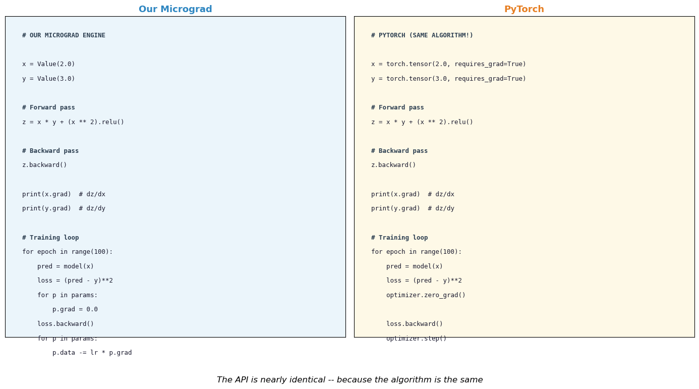
The code structure is almost identical.
PyTorch wraps the same reverse-mode AD in optimized C++/CUDA kernels.

Show code cell source Hide code cell source

# Visualize the evolution of AD frameworks

fig, ax = plt.subplots(figsize=(14, 5))

events = [
    (1970, 'Linnainmaa\nReverse-mode AD', '#E74C3C', 0.7),
    (1982, 'Werbos\nAD for NNs', '#E74C3C', -0.7),
    (1986, 'Rumelhart et al.\nBackpropagation', '#E74C3C', 0.7),
    (2000, 'Griewank\nEvaluating\nDerivatives', '#F39C12', -0.7),
    (2010, 'Theano\nTensor AD', '#3498DB', 0.7),
    (2015, 'TensorFlow\nStatic graphs', '#3498DB', -0.7),
    (2017, 'PyTorch\nDynamic graphs', '#3498DB', 0.7),
    (2018, 'Baydin et al.\nAD Survey', '#F39C12', -0.7),
    (2020, 'JAX\nFunctional AD', '#3498DB', 0.7),
]

ax.axhline(0, color='#2C3E50', linewidth=2, zorder=1)

for year, label, color, y_offset in events:
    ax.plot(year, 0, 'o', markersize=10, color=color, zorder=3,
            markeredgecolor='black', markeredgewidth=1.5)
    ax.annotate(label, xy=(year, 0), xytext=(year, y_offset),
                fontsize=8, ha='center', va='center',
                bbox=dict(boxstyle='round,pad=0.3', facecolor=color, alpha=0.15),
                arrowprops=dict(arrowstyle='->', color=color, lw=1.5))

ax.set_xlim(1965, 2025)
ax.set_ylim(-1.3, 1.3)
ax.set_xlabel('Year', fontsize=12)
ax.set_title('Timeline of Automatic Differentiation', fontsize=13)
ax.set_yticks([])
ax.grid(True, alpha=0.2, axis='x')

from matplotlib.patches import Patch
legend_elements = [
    Patch(facecolor='#E74C3C', alpha=0.3, label='Theory'),
    Patch(facecolor='#3498DB', alpha=0.3, label='Frameworks'),
    Patch(facecolor='#F39C12', alpha=0.3, label='Textbooks/Surveys'),
]
ax.legend(handles=legend_elements, loc='upper left', fontsize=10)

plt.tight_layout()
plt.show()

print("Reverse-mode AD was invented in 1970 -- 47 years before PyTorch!")

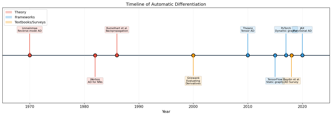
Reverse-mode AD was invented in 1970 -- 47 years before PyTorch!

A Deeper Look: Dynamic vs Static Graphs

There are two philosophies for building computation graphs in AD frameworks:

Static graphs (TensorFlow 1.x, Theano): The user defines the computation graph first, then executes it. The graph is fixed before any data flows through it. This allows aggressive compile-time optimization but makes debugging difficult and prohibits data-dependent control flow (e.g., if loss > threshold).

Dynamic graphs (PyTorch, JAX, our Value class): The graph is constructed on-the-fly during the forward pass. Each time you compute a + b, a new node is added to the graph. This is called “define-by-run” and is the approach we implemented: our Value.__add__ creates a new Value node with _prev pointing to its inputs.

Tip

In the next chapter, we will switch to PyTorch for training neural networks. Now you know what loss.backward() does under the hood – it is exactly the topological sort and reverse traversal that our Value.backward() performs, just operating on tensors instead of scalars, with C++ and CUDA acceleration.

Exercises

Exercise 28.1. Add sigmoid to the Value class:

\[\sigma(x) = \frac{1}{1 + e^{-x}}, \qquad \sigma'(x) = \sigma(x)(1 - \sigma(x))\]

Verify your implementation using numerical gradient checking.

Exercise 28.2. Implement forward-mode AD for the function \(f(x, y) = x^2 y + \sin(xy)\). Use dual numbers: represent each value as \((v, \dot{v})\) where \(\dot{v} = \partial v / \partial x_i\). Compute \(\partial f / \partial x\) in one forward pass, then \(\partial f / \partial y\) in a second pass. Compare the cost with reverse mode.

Exercise 28.3. Draw the computational graph (on paper or using matplotlib) for the function \(f(x, y, z) = (x + y) \cdot z + \exp(x \cdot z)\). Label all nodes with their values for \(x = 1, y = 2, z = -1\). Then perform the backward pass manually, computing \(\partial f / \partial x\), \(\partial f / \partial y\), \(\partial f / \partial z\). Verify with our Value class.

Exercise 28.4. Our Value class stores the entire computation graph in memory (via _prev). For very deep networks, this can cause memory issues. Research “gradient checkpointing” (Chen et al., 2016): the idea of discarding intermediate activations during the forward pass and recomputing them during the backward pass. What is the time-memory trade-off?

Exercise 28.5. Extend the MLP class to support a configurable number of hidden layers and different activation functions per layer. Train a deeper network (e.g., 2 -> 8 -> 8 -> 1) on the XOR problem. Does depth help or hurt for this simple task?

Exercise 28.6. Modify our autograd engine to also track the computation count: how many elementary operations are performed in the forward pass, and how many in the backward pass. Verify empirically that the backward pass costs at most a small constant multiple of the forward pass (Griewank’s “cheap gradient principle”).