Chapter 29: From Micrograd to PyTorch – Tensors, Autograd, and nn.Module

Chapter 29: From Micrograd to PyTorch – Tensors, Autograd, and nn.Module#

In the previous chapter, we built a reverse-mode automatic differentiation engine from scratch. Our Value class operated on scalars – each number was individually tracked through a computational graph, and gradients flowed backward one scalar at a time. This was conceptually illuminating but computationally impractical: real neural networks have millions of parameters, and operating on them one-by-one would be absurdly slow.

PyTorch extends the same idea to multi-dimensional arrays – tensors – with GPU acceleration. The gradient tape we built by hand in Chapter 28 is precisely what torch.autograd does under the hood, but on tensors of arbitrary shape, with hundreds of optimized backward kernels, and with optional CUDA parallelism.

This chapter bridges the gap between our educational micrograd engine and the industrial-strength framework we will use for the rest of the course.

PyTorch version: 2.7.0
CUDA available: False

29.1 Historical Context: The Rise of Deep Learning Frameworks#

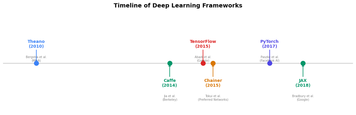
The history of neural network software follows a clear trajectory from manual gradient derivation toward fully automatic, hardware-accelerated differentiation.

Theano (2010). Developed at the Montreal Institute for Learning Algorithms (MILA) under Yoshua Bengio, Theano was the first widely adopted framework to combine symbolic differentiation with GPU compilation. Users defined computation graphs symbolically, then Theano compiled them into optimized CUDA code. The landmark paper by Bergstra et al. (2010) introduced the paradigm of “define-then-run” that would dominate for years.

Caffe (2014). Yangqing Jia’s framework from Berkeley emphasized speed and modularity for convolutional networks. Caffe’s prototxt configuration files made it easy to define standard architectures without writing code, but this rigidity made experimentation with novel architectures difficult.

TensorFlow (2015). Google’s framework, described by Abadi et al. (2016), adopted Theano’s define-then-run paradigm with industrial-scale engineering. Its static graph approach offered deployment advantages but made debugging notoriously painful – Python served merely as a graph-construction language, with actual execution happening in a separate C++ runtime.

PyTorch (2017). Paszke et al. introduced a radically different approach: define-by-run (also called “eager execution”). Instead of building a static graph and then executing it, PyTorch builds the computational graph dynamically as operations execute. This means standard Python control flow (if, for, while) works naturally inside models – a crucial advantage for research. The framework descended from Torch7 (a Lua-based system) and drew on the ideas of Chainer (2015), which pioneered define-by-run in Python.

JAX (2018). Google’s response to PyTorch, led by Bradbury et al., combined NumPy-compatible syntax with functional transformations (jit, grad, vmap). JAX compiles Python+NumPy programs via XLA, offering both eager and compiled modes.

The Convergence

By 2019, TensorFlow added eager execution (TF 2.0), and PyTorch added compilation (torch.jit). The frameworks converged toward a common design: eager by default for development, with optional compilation for deployment. As of 2024, PyTorch dominates research (>80% of ML papers) while TensorFlow retains a significant deployment footprint.

../_images/58fb4b158b71d2ab011c9edb6ad8cc164db20affa9406c89718dfeeee30ba3d4.png

29.2 Tensors as Generalized Arrays#

A tensor in PyTorch is a multi-dimensional array, conceptually identical to NumPy’s ndarray but with two critical additions:

Automatic differentiation support – tensors can track operations for gradient computation.
Device placement – tensors can live on CPU or GPU, enabling hardware acceleration.

The mathematical terminology is precise: a scalar is a 0-dimensional tensor, a vector is 1-dimensional, a matrix is 2-dimensional, and higher-rank objects are simply called tensors. PyTorch uses the same convention.

Creating Tensors#

# --- Tensor creation ---

# From Python lists
t1 = torch.tensor([1.0, 2.0, 3.0])
print(f'From list:    {t1}, dtype={t1.dtype}, shape={t1.shape}')

# From NumPy (shares memory -- no copy!)
arr = np.array([[1, 2], [3, 4]], dtype=np.float32)
t2 = torch.from_numpy(arr)
print(f'From NumPy:   {t2.shape}, dtype={t2.dtype}')

# Back to NumPy
arr_back = t2.numpy()
print(f'Back to NumPy: same object? {np.shares_memory(arr, arr_back)}')

# Standard constructors
t_zeros = torch.zeros(2, 3)
t_ones = torch.ones(2, 3)
t_rand = torch.randn(2, 3)  # standard normal
t_eye = torch.eye(3)

print(f'\nzeros(2,3):\n{t_zeros}')
print(f'\neye(3):\n{t_eye}')

From list:    tensor([1., 2., 3.]), dtype=torch.float32, shape=torch.Size([3])
From NumPy:   torch.Size([2, 2]), dtype=torch.float32
Back to NumPy: same object? True

zeros(2,3):
tensor([[0., 0., 0.],
        [0., 0., 0.]])

eye(3):
tensor([[1., 0., 0.],
        [0., 1., 0.],
        [0., 0., 1.]])

Data Types and Device#

# --- Data types ---
t_int = torch.tensor([1, 2, 3])          # default: int64
t_float = torch.tensor([1.0, 2.0, 3.0])  # default: float32
t_double = torch.tensor([1.0, 2.0], dtype=torch.float64)

print(f'Integer tensor: dtype={t_int.dtype}')
print(f'Float tensor:   dtype={t_float.dtype}')
print(f'Double tensor:  dtype={t_double.dtype}')

# Type casting
t_cast = t_int.float()  # int64 -> float32
print(f'After .float(): dtype={t_cast.dtype}')

# Device (CPU by default, GPU if available)
device = torch.device('cuda' if torch.cuda.is_available() else 'cpu')
print(f'\nUsing device: {device}')
t_device = t_float.to(device)
print(f'Tensor on {t_device.device}')

Integer tensor: dtype=torch.int64
Float tensor:   dtype=torch.float32
Double tensor:  dtype=torch.float64
After .float(): dtype=torch.float32

Using device: cpu
Tensor on cpu

Tensor Operations#

PyTorch tensors support the same broadcasting and vectorized operations as NumPy. Every operation builds a node in the computational graph (when requires_grad=True).

# --- Basic operations ---
a = torch.tensor([[1.0, 2.0], [3.0, 4.0]])
b = torch.tensor([[5.0, 6.0], [7.0, 8.0]])

print('Element-wise addition:')
print(a + b)

print('\nMatrix multiplication:')
print(a @ b)

print('\nBroadcasting (matrix + scalar):')
print(a + 10)

print('\nReduction (sum along axis 1):')
print(a.sum(dim=1))

print('\nReshape:')
print(a.view(4))  # flatten
print(a.view(1, 4))  # row vector

Element-wise addition:
tensor([[ 6.,  8.],
        [10., 12.]])

Matrix multiplication:
tensor([[19., 22.],
        [43., 50.]])

Broadcasting (matrix + scalar):
tensor([[11., 12.],
        [13., 14.]])

Reduction (sum along axis 1):
tensor([3., 7.])

Reshape:
tensor([1., 2., 3., 4.])
tensor([[1., 2., 3., 4.]])

29.3 Autograd on Tensors#

In Chapter 28, we built a Value class that tracked operations on scalars and accumulated gradients via reverse-mode AD. PyTorch’s autograd does exactly the same thing, but on tensors.

The key API:

Set requires_grad=True on a tensor to start tracking operations.
Call .backward() on a scalar loss to compute all gradients.
Access gradients via the .grad attribute.

Connection to Chapter 28

Recall that our micrograd Value stored self.grad and self._backward for each node. PyTorch tensors have the same structure: each tensor with requires_grad=True stores a .grad tensor and a .grad_fn pointing to the backward function of the operation that created it.

Replicating the Micrograd Example#

In Chapter 28, we computed gradients of \(f(x, y) = (x + y) \cdot y\) at \(x = 2, y = 3\). Let us verify that PyTorch produces the same result.

# --- Replicating ch28's micrograd example ---

# In ch28, we computed: f(x,y) = (x + y) * y
# df/dx = y = 3, df/dy = x + 2y = 2 + 6 = 8

x = torch.tensor(2.0, requires_grad=True)
y = torch.tensor(3.0, requires_grad=True)

# Forward pass
f = (x + y) * y
print(f'f(2, 3) = {f.item():.1f}')

# Backward pass
f.backward()

print(f'df/dx = {x.grad.item():.1f}  (expected: 3.0)')
print(f'df/dy = {y.grad.item():.1f}  (expected: 8.0)')

# Verify: the grad_fn shows the last operation
print(f'\nf.grad_fn = {f.grad_fn}')

f(2, 3) = 15.0

df/dx = 3.0  (expected: 3.0)
df/dy = 8.0  (expected: 8.0)

f.grad_fn = <MulBackward0 object at 0x136605390>

Exact Match

The gradients \(\frac{\partial f}{\partial x} = 3\) and \(\frac{\partial f}{\partial y} = 8\) match exactly what our hand-built Value class computed in Chapter 28. This is not a coincidence – both implement the same reverse-mode AD algorithm. The difference is that PyTorch’s implementation is written in C++ and operates on tensors of arbitrary shape.

Autograd with Tensors (not just scalars)#

The real power of PyTorch emerges when we compute gradients of tensor expressions. Consider a simple linear regression loss:

# --- Autograd on tensor operations ---
torch.manual_seed(42)

# Parameters
W = torch.randn(3, 2, requires_grad=True)
b = torch.randn(2, requires_grad=True)

# Input batch (4 samples, 3 features)
X = torch.randn(4, 3)
y_true = torch.randn(4, 2)

# Forward pass: linear transformation + MSE loss
y_pred = X @ W + b             # (4, 2)
loss = ((y_pred - y_true)**2).mean()

print(f'Loss: {loss.item():.4f}')
print(f'W.grad before backward: {W.grad}')

# Backward pass
loss.backward()

print(f'\nW.grad after backward (shape {W.grad.shape}):')
print(W.grad)
print(f'\nb.grad after backward: {b.grad}')

Loss: 4.3729
W.grad before backward: None

W.grad after backward (shape torch.Size([3, 2])):
tensor([[ 1.5130, -0.1619],
        [ 0.9877, -0.4371],
        [-2.4168, -0.0719]])

b.grad after backward: tensor([ 2.0992, -0.8098])

Important: Zero Gradients

PyTorch accumulates gradients by default. If you call .backward() twice without zeroing, gradients will be summed. This is occasionally useful (e.g., gradient accumulation across mini-batches) but usually a source of bugs. Always call optimizer.zero_grad() or manually set .grad = None before each backward pass.

# --- Demonstration: gradient accumulation trap ---
p = torch.tensor(2.0, requires_grad=True)

# First backward
loss1 = p ** 2
loss1.backward()
print(f'After 1st backward: p.grad = {p.grad.item()}')

# Second backward WITHOUT zeroing
loss2 = p ** 2
loss2.backward()
print(f'After 2nd backward (accumulated!): p.grad = {p.grad.item()}')

# Fix: zero the gradient
p.grad = None
loss3 = p ** 2
loss3.backward()
print(f'After zeroing + 3rd backward: p.grad = {p.grad.item()}')

After 1st backward: p.grad = 4.0
After 2nd backward (accumulated!): p.grad = 8.0
After zeroing + 3rd backward: p.grad = 4.0

29.4 nn.Module: Building Neural Networks#

In Chapter 28, we built a Neuron class from Value objects, then composed neurons into Layer and MLP classes. PyTorch provides an analogous but more powerful abstraction: nn.Module.

An nn.Module is any differentiable building block:

It has parameters (learnable tensors registered via nn.Parameter).
It defines a forward() method that computes the output.
It automatically collects parameters from sub-modules.

The Module Hierarchy

Just as our micrograd MLP contained Layer objects which contained Neuron objects, a PyTorch nn.Module can contain other nn.Module instances as attributes. The framework automatically discovers all parameters recursively via model.parameters().

XOR Network as nn.Module#

Let us solve the XOR problem – the same task from Chapters 8 and 28 – using nn.Module. We use the same 2-2-1 architecture.

class XORNet(nn.Module):
    """A 2-2-1 network for XOR, matching the ch28 micrograd architecture."""
    
    def __init__(self):
        super().__init__()
        self.hidden = nn.Linear(2, 2)   # 2 inputs -> 2 hidden
        self.output = nn.Linear(2, 1)   # 2 hidden -> 1 output
    
    def forward(self, x):
        x = torch.tanh(self.hidden(x))
        x = torch.tanh(self.output(x))
        return x

# Inspect the model
torch.manual_seed(42)
model = XORNet()
print(model)
print(f'\nTotal parameters: {sum(p.numel() for p in model.parameters())}')
print('\nParameter details:')
for name, param in model.named_parameters():
    print(f'  {name}: shape={param.shape}, requires_grad={param.requires_grad}')

XORNet(
  (hidden): Linear(in_features=2, out_features=2, bias=True)
  (output): Linear(in_features=2, out_features=1, bias=True)
)

Total parameters: 9

Parameter details:
  hidden.weight: shape=torch.Size([2, 2]), requires_grad=True
  hidden.bias: shape=torch.Size([2]), requires_grad=True
  output.weight: shape=torch.Size([1, 2]), requires_grad=True
  output.bias: shape=torch.Size([1]), requires_grad=True

# --- Train XOR network ---
torch.manual_seed(42)
model = XORNet()

# XOR dataset (matching ch28)
X_xor = torch.tensor([[0.0, 0.0], [0.0, 1.0], [1.0, 0.0], [1.0, 1.0]])
Y_xor = torch.tensor([[-1.0], [1.0], [1.0], [-1.0]])  # tanh targets

optimizer = torch.optim.SGD(model.parameters(), lr=0.5)
losses = []

for epoch in range(500):
    # Forward pass
    pred = model(X_xor)
    loss = ((pred - Y_xor) ** 2).mean()
    
    # Backward pass
    optimizer.zero_grad()
    loss.backward()
    optimizer.step()
    
    losses.append(loss.item())

# Final predictions
with torch.no_grad():
    final_pred = model(X_xor)

print('XOR Training Results:')
print(f'Final loss: {losses[-1]:.6f}')
print()
for i in range(4):
    x_str = f'({X_xor[i, 0]:.0f}, {X_xor[i, 1]:.0f})'
    print(f'  Input {x_str} -> pred={final_pred[i, 0]:+.4f}, target={Y_xor[i, 0]:+.0f}')

XOR Training Results:
Final loss: 0.001538

  Input (0, 0) -> pred=-0.9639, target=-1
  Input (0, 1) -> pred=+0.9570, target=+1
  Input (1, 0) -> pred=+0.9554, target=+1
  Input (1, 1) -> pred=-0.9686, target=-1

../_images/2543af4a0fd812e7fabc3ec417d2c7449a78630c0bbe3616014619cdbc31a0be.png

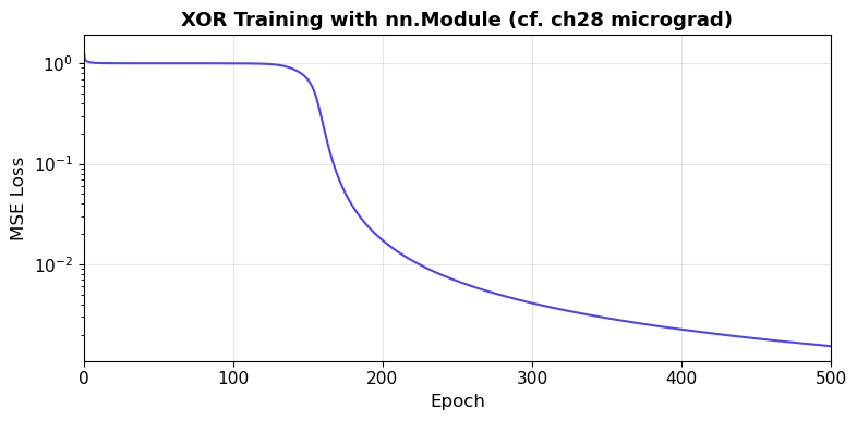
Micrograd vs. PyTorch: Same Algorithm, Different Scale

Compare the training loop above with the one in Chapter 28. The structure is identical: forward pass, loss computation, backward pass, parameter update. The only differences are:

We operate on batched tensors instead of individual Value scalars.
optimizer.zero_grad() replaces our manual p.grad = 0 loop.
optimizer.step() replaces our manual p.data -= lr * p.grad loop.
torch.no_grad() context manager replaces our careful avoidance of gradient tracking during evaluation.

29.5 Common Modules: nn.Linear, nn.ReLU, nn.Sequential#

PyTorch provides a rich library of pre-built modules. The most fundamental are:

Module	Description	Parameters
`nn.Linear(in, out)`	Affine transformation \(y = xW^T + b\)	\(W \in \mathbb{R}^{\text{out} \times \text{in}}\), \(b \in \mathbb{R}^{\text{out}}\)
`nn.ReLU()`	Rectified linear unit \(\max(0, x)\)	None
`nn.Tanh()`	Hyperbolic tangent	None
`nn.Sigmoid()`	Logistic function \(\sigma(x) = \frac{1}{1 + e^{-x}}\)	None
`nn.Sequential(...)`	Chain modules in order	Inherited

XOR with nn.Sequential#

For simple feed-forward architectures, nn.Sequential eliminates the need to write a custom forward() method:

# --- XOR with nn.Sequential ---
torch.manual_seed(42)

model_seq = nn.Sequential(
    nn.Linear(2, 8),
    nn.ReLU(),
    nn.Linear(8, 1),
)

print(model_seq)
print(f'\nTotal parameters: {sum(p.numel() for p in model_seq.parameters())}')

# XOR data (0/1 targets for ReLU-based network)
X_xor = torch.tensor([[0.0, 0.0], [0.0, 1.0], [1.0, 0.0], [1.0, 1.0]])
Y_xor = torch.tensor([[0.0], [1.0], [1.0], [0.0]])

optimizer = torch.optim.Adam(model_seq.parameters(), lr=0.01)
loss_fn = nn.MSELoss()

for epoch in range(1000):
    pred = model_seq(X_xor)
    loss = loss_fn(pred, Y_xor)
    optimizer.zero_grad()
    loss.backward()
    optimizer.step()

# Results
with torch.no_grad():
    final_pred = model_seq(X_xor)

print('\nXOR with Sequential + ReLU:')
for i in range(4):
    x_str = f'({X_xor[i, 0]:.0f}, {X_xor[i, 1]:.0f})'
    print(f'  Input {x_str} -> pred={final_pred[i, 0]:.4f}, target={Y_xor[i, 0]:.0f}')

Sequential(
  (0): Linear(in_features=2, out_features=8, bias=True)
  (1): ReLU()
  (2): Linear(in_features=8, out_features=1, bias=True)
)

Total parameters: 33

XOR with Sequential + ReLU:
  Input (0, 0) -> pred=0.0000, target=0
  Input (0, 1) -> pred=1.0000, target=1
  Input (1, 0) -> pred=1.0000, target=1
  Input (1, 1) -> pred=0.0000, target=0

Custom Module vs. Sequential: When to Use Which#

Rule of Thumb

Use nn.Sequential for straightforward feed-forward architectures where data flows linearly through layers. Write a custom nn.Module when you need:

Skip connections (ResNet)
Multiple inputs or outputs
Conditional computation
Custom logic in the forward pass

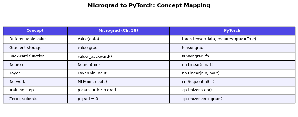
The Forward-Backward Duality#

Every nn.Module defines a forward() method. PyTorch’s autograd automatically provides the corresponding backward computation. This is the industrial realization of the principle we explored in Chapter 28: if you can evaluate a function, you can differentiate it.

The following diagram shows the correspondence between our micrograd building blocks and their PyTorch equivalents:

../_images/ba6590c8a5af9807b53a44900c83198809a9d546ecf88ee21c0c8992a1e0f151.png

Exercises#

Exercise 29.1. Create a 3D tensor of shape \((2, 3, 4)\) filled with random integers between 0 and 9. Print its shape, dtype, device, and the total number of elements. Convert it to float32 and verify the dtype changed.

Exercise 29.2. Using PyTorch autograd, compute the gradient of \(f(x) = \frac{e^{2x}}{(1 + e^{2x})^2}\) at \(x = 1\). Verify your answer by comparing with the analytical derivative (note that \(f(x) = \sigma'(2x) \cdot 2\) where \(\sigma\) is the sigmoid function).

Exercise 29.3. Build a custom nn.Module for a network with skip connections: the architecture should be \(y = \text{ReLU}(W_2 \cdot \text{ReLU}(W_1 x + b_1) + b_2) + x\). This cannot be expressed as nn.Sequential. Test it on a random input of shape \((4, 8)\).

Exercise 29.4. Demonstrate the gradient accumulation issue: create a parameter \(\theta = 3.0\), compute \(\nabla_\theta (\theta^3)\) twice without zeroing, and show that the gradient doubles. Then fix it with param.grad = None.

Exercise 29.5. Rewrite the XORNet class to use nn.ReLU activations instead of torch.tanh, with \([0, 1]\) targets instead of \([-1, 1]\). How many hidden units are needed for reliable convergence? Experiment with hidden sizes 2, 4, 8, and 16.

References.

Paszke, A., Gross, S., Massa, F., et al. (2019). “PyTorch: An Imperative Style, High-Performance Deep Learning Library.” Advances in Neural Information Processing Systems 32.
Bergstra, J., Breuleux, O., Bastien, F., et al. (2010). “Theano: A CPU and GPU Math Compiler in Python.” Proc. SciPy 2010.
Abadi, M., Barham, P., Chen, J., et al. (2016). “TensorFlow: A System for Large-Scale Machine Learning.” 12th USENIX Symposium on OSDI.
Bradbury, J., Frostig, R., Hawkins, P., et al. (2018). “JAX: Composable transformations of Python+NumPy programs.” GitHub repository.
Karpathy, A. (2020). “micrograd: A tiny scalar-valued autograd engine.” GitHub repository.