Chapter 38: Attention Variants

In Chapter 37 you implemented the attention mechanism of Bahdanau, Cho & Bengio (2014) — the first variant ever published. The score function was additive:

\[ e_{ij} \;=\; v_a^\top \tanh\!\bigl(W_a [s_{i-1}; h_j]\bigr). \]

It works beautifully but it has two costs: a small MLP per (query, key) pair, and an extra parameter matrix \(W_a\). A year later, Luong, Pham, and Manning (2015) asked a deceptively simple question: do we really need that MLP, or can we just take a dot product?

This chapter develops the design space of attention scores. We will:

• compare additive, dot-product, multiplicative (general), and scaled-dot-product attention;

• derive from first principles why we need the \(\sqrt{d_k}\) normalisation that defines the modern Transformer — the answer connects directly back to Chapter 17’s vanishing-gradient analysis;

• visualise softmax saturation as \(d_k\) grows, with and without scaling;

• mention coverage mechanisms (See, Liu, Manning 2017) as a way to fight repetition.

Original paper: Luong, Pham, Manning. Effective Approaches to Attention-based Neural Machine Translation. EMNLP 2015 (arXiv:1508.04025).

38.1 The Four Score Functions

Write the decoder query as \(s \in \mathbb{R}^{d_s}\) and an encoder state as \(h \in \mathbb{R}^{d_h}\). Every attention variant is just a different choice of score function \(e(s, h) \in \mathbb{R}\).

Variant	Score \(e(s, h)\)	Parameters	Cost per pair
Additive (Bahdanau)	\(v_a^\top \tanh(W_a [s; h])\)	\(W_a \in \mathbb{R}^{d_a \times (d_s+d_h)}\), \(v_a \in \mathbb{R}^{d_a}\)	\(O(d_a (d_s + d_h))\)
Dot product	\(s^\top h\)	none (requires \(d_s = d_h\))	\(O(d)\)
Multiplicative	\(s^\top W_g h\)	\(W_g \in \mathbb{R}^{d_s \times d_h}\)	\(O(d_s d_h)\)
Scaled dot product	\(s^\top h / \sqrt{d_k}\)	none	\(O(d)\)

Two observations.

1. Dot product is by far the cheapest. It has no parameters and reduces to a single matrix multiplication \(S K^\top\) when batched. This is why every modern Transformer uses it.

2. Multiplicative attention is dot-product on a projected key. The projection \(K' = K W_g^\top\) can absorb the \(W_g\). So multiplicative is really the same as dot product after a learnable rotation.

But there is a catch — and it is exactly the catch that motivated the \(\sqrt{d_k}\) scaling. Section 38.3 will derive it from scratch.

import sys, os
sys.path.insert(0, os.path.abspath('.'))

import math, random
import torch
import torch.nn as nn
import torch.nn.functional as F
import numpy as np
import matplotlib.pyplot as plt

from utils import VOCAB_SIZE, PAD, SOS, EOS, ITOS, encode, decode, make_batch, accuracy

torch.manual_seed(0); random.seed(0)
device = torch.device('cpu')

def attention_scores(s, H, kind='dot', d_k=None, W_g=None, W_a=None, v_a=None):
    """Compute attention weights alpha (B, T) for one decoder step.

    s: (B, d_s)        decoder query
    H: (B, T, d_h)     encoder keys/values
    """
    if kind == 'dot':
        e = torch.bmm(H, s.unsqueeze(-1)).squeeze(-1)            # (B, T)
    elif kind == 'general':
        sW = s @ W_g                                              # (B, d_h)
        e = torch.bmm(H, sW.unsqueeze(-1)).squeeze(-1)
    elif kind == 'scaled':
        e = torch.bmm(H, s.unsqueeze(-1)).squeeze(-1) / math.sqrt(d_k)
    elif kind == 'additive':
        # v^T tanh(W [s; h])
        s_exp = s.unsqueeze(1).expand(-1, H.size(1), -1)         # (B, T, d_s)
        cat = torch.cat([s_exp, H], dim=-1)                      # (B, T, d_s+d_h)
        e = v_a(torch.tanh(W_a(cat))).squeeze(-1)                # (B, T)
    return F.softmax(e, dim=-1), e

A worked example: all four scores on one \((s, h)\) pair

Before plotting anything, let us compute each variant by hand on a tiny shared example so the formulas stop being symbolic. Take \(d_s = d_h = d_a = 4\) and a single key (so we can read all numbers).

\[\begin{split} s = \begin{pmatrix} 1.0 \\ -0.5 \\ 0.3 \\ 0.8 \end{pmatrix}, \qquad h = \begin{pmatrix} 0.6 \\ 0.2 \\ -0.4 \\ 1.0 \end{pmatrix}. \end{split}\]

The dot product is \(s^\top h = 0.6 - 0.1 - 0.12 + 0.8 = 1.18\). The scaled version divides by \(\sqrt{4} = 2\), giving \(0.59\). The general (multiplicative) score depends on \(W_g\), and the additive score depends on \((W_a, v_a)\). The cell below evaluates all four on the same random parameters and prints the intermediate quantities so you can trace the arithmetic.

torch.manual_seed(11)
d = 4
s = torch.tensor([1.0, -0.5, 0.3, 0.8])
h = torch.tensor([0.6,  0.2, -0.4, 1.0])

# Random parameters for the parametrised variants.
W_g = torch.randn(d, d) * 0.3
W_a = torch.randn(d, 2 * d) * 0.3   # maps [s; h] -> R^d
v_a = torch.randn(d) * 0.3

# 1. Dot product
e_dot = (s * h).sum().item()

# 2. Scaled dot product
e_scl = e_dot / math.sqrt(d)

# 3. General / multiplicative: s^T W_g h
sW   = s @ W_g                    # (d,)
e_gen = (sW * h).sum().item()

# 4. Additive / Bahdanau: v_a^T tanh(W_a [s; h])
cat   = torch.cat([s, h])         # (2d,)
hid   = torch.tanh(W_a @ cat)     # (d,)
e_add = (v_a * hid).item() if v_a.dim() == 0 else (v_a @ hid).item()

print(f'dot                e = {e_dot:+.4f}')
print(f'scaled dot         e = {e_scl:+.4f}   (= dot / sqrt({d}))')
print(f'general (s W_g h)  e = {e_gen:+.4f}   intermediate s W_g = {sW.numpy().round(3)}')
print(f'additive           e = {e_add:+.4f}   tanh(W_a[s;h]) = {hid.numpy().round(3)}')

dot                e = +1.1800
scaled dot         e = +0.5900   (= dot / sqrt(4))
general (s W_g h)  e = +0.3471   intermediate s W_g = [ 0.166  0.57  -0.183  0.06 ]
additive           e = -0.6569   tanh(W_a[s;h]) = [-0.63   0.659 -0.101  0.877]

Two things to notice. First, general attention is genuinely a different score from plain dot — the matrix \(W_g\) rotates and rescales \(s\) before it meets \(h\). Second, additive attention is the only one that can be non-monotone in \(s^\top h\) because the \(\tanh\) non-linearity sits between the two vectors. This is exactly the extra expressivity hinted at in Exercise 38.6.

38.2 Why Just Take a Dot Product?

The dot product \(s^\top h\) is large when \(s\) and \(h\) point in similar directions. So if the encoder learns to place the relevant state near the current decoder query, the dot product is automatically large. No explicit alignment network required — the encoder and decoder learn to agree on a coordinate system.

This is geometrically beautiful and computationally cheap. It is also the seed of self-attention (Chapter 39). But the geometry has a problem at high dimension.

Historical context: what problem was Luong solving?

Bahdanau, Cho, Bengio (2014, arXiv:1409.0473) had just shown that content-based attention obliterated fixed-vector encoder-decoders on WMT’14 English-French. But their additive score required, for every \((i, j)\) pair, a forward pass through a small MLP. On a 50-token source sentence and a 50-token target this meant \(50 \times 50 = 2{,}500\) extra MLP evaluations per training example, and back-prop through all of them.

Luong, Pham, Manning (EMNLP 2015, arXiv:1508.04025) were optimising for WMT’15 English-German, a harder task with longer sentences. They asked: can we replace the MLP with a bilinear form \(s^\top W_g h\) (“general”), or even nothing at all (“dot”)? Their empirical answer: yes, dot-product attention matches additive on BLEU when the hidden dimension is moderate, and is dramatically faster because \(S K^\top\) is one matmul. That single observation is the bridge from RNN attention to the Transformer.

38.3 The \(\sqrt{d_k}\) Scaling — Derivation

Suppose \(s\) and \(h\) are random vectors in \(\mathbb{R}^{d_k}\) with i.i.d. components of mean \(0\) and variance \(1\). What is the variance of their dot product?

\[ s^\top h \;=\; \sum_{k=1}^{d_k} s_k h_k. \]

Each term has mean \(0\) and variance \(\mathrm{Var}(s_k h_k) = \mathbb{E}[s_k^2]\mathbb{E}[h_k^2] = 1 \cdot 1 = 1\) (using independence and \(\mathbb{E}[s_k] = \mathbb{E}[h_k] = 0\)). The \(d_k\) terms are independent, so

\[ \boxed{\quad \mathrm{Var}\!\left(s^\top h\right) \;=\; d_k. \quad} \]

So the scale of the score grows like \(\sqrt{d_k}\). For \(d_k = 64\) scores have standard deviation \(8\); for \(d_k = 1024\) they have standard deviation \(32\).

Now feed those scores through a softmax. The softmax saturates: gradients vanish. This is exactly the failure mode you analysed for sigmoid in Chapter 17 — when the input to a softmax/sigmoid is large in magnitude, the output becomes near 1 or 0 and the derivative collapses. Recall from Chapter 17 that \(\sigma'(x) \le 1/4\), with equality at \(x = 0\) and exponential decay outside.

The fix is to scale the scores back to unit variance:

\[ e_{ij} \;=\; \frac{s^\top h}{\sqrt{d_k}}. \]

Vaswani et al. (2017) report this single change makes Transformer training stable at the scales they wanted. We will see why visually in the next cells.

Why does softmax saturation kill gradients? (the Ch 17 link, made quantitative)

The softmax \(p_j = e^{e_j} / \sum_k e^{e_k}\) has Jacobian

\[ \frac{\partial p_i}{\partial e_j} \;=\; p_i(\delta_{ij} - p_j). \]

When the distribution is uniform, \(p_i = 1/T\), so \(|\partial p_i / \partial e_j| = (1/T)(1 - 1/T) \approx 1/T\) — the gradient is shared among all keys.

When the distribution is one-hot, say \(p_1 \to 1\) and \(p_{j>1} \to 0\), the entire Jacobian goes to zero: \(p_1(1 - p_1) \to 0\) and \(p_i p_j \to 0\) for \(i \neq j\). No information about which key was right can flow back through the score.

Compare this to Chapter 17’s sigmoid analysis: \(\sigma'(x) = \sigma(x)(1 - \sigma(x)) \le 1/4\), with the bound saturated at \(x = 0\). Softmax is the same product-of-probabilities structure in a higher-dimensional disguise. The \(\sqrt{d_k}\) scaling is to attention what centring activations near zero (or LayerNorm) is to sigmoid networks: it keeps the input to the saturating non-linearity in its linear regime.

The next cell visualises this directly — gradient norm of the softmax output with respect to the largest score, as a function of how peaked the distribution is.

# Sweep score temperature; measure gradient norm of softmax output.
T_keys = 16
base = torch.linspace(-1, 1, T_keys)
scales = np.linspace(0.1, 20, 60)
grad_norms = []
for sc in scales:
    e = (base * sc).clone().requires_grad_(True)
    p = F.softmax(e, dim=-1)
    # Surrogate scalar: pick the top probability and back-prop.
    p.max().backward()
    grad_norms.append(e.grad.norm().item())

fig, ax = plt.subplots(figsize=(7, 3.5))
ax.plot(scales, grad_norms, color='#dc2626', lw=2)
ax.set(xlabel='score scale (proportional to $\\sqrt{d_k}$)',
       ylabel=r'$\|\nabla_e \, \max_j p_j\|_2$',
       title='Softmax gradient collapses as scores grow')
ax.grid(alpha=0.3)
ax.axvline(1.0, ls='--', color='gray', alpha=0.6)
ax.text(1.1, ax.get_ylim()[1] * 0.85, 'unit-variance scores\n(what scaling restores)',
        fontsize=8, color='gray')
plt.tight_layout(); plt.show()

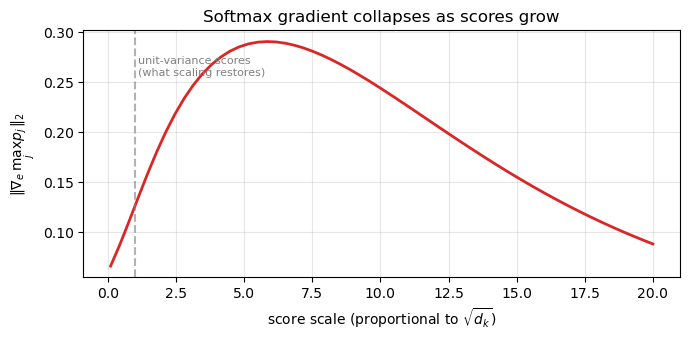
The gradient norm peaks near unit-variance scores and falls to near-zero by score scale \(\approx 10\). Without scaling, \(d_k = 100\) already puts you at score scale \(\sqrt{100} = 10\) — the saturating regime. That is the entire reason the \(1/\sqrt{d_k}\) factor exists.

# Confirm the variance derivation empirically.
for d in [4, 16, 64, 256, 1024]:
    s = torch.randn(10000, d)
    h = torch.randn(10000, d)
    dp = (s * h).sum(-1)
    print(f'd_k = {d:5d}  mean={dp.mean().item(): .3f}  '
          f'std (empirical) = {dp.std().item():6.2f}  '
          f'sqrt(d) = {math.sqrt(d):6.2f}')

d_k =     4  mean= 0.004  std (empirical) =   1.98  sqrt(d) =   2.00
d_k =    16  mean= 0.018  std (empirical) =   4.05  sqrt(d) =   4.00
d_k =    64  mean=-0.106  std (empirical) =   7.87  sqrt(d) =   8.00
d_k =   256  mean=-0.198  std (empirical) =  16.00  sqrt(d) =  16.00

d_k =  1024  mean=-0.568  std (empirical) =  31.99  sqrt(d) =  32.00

Empirical \(\mathrm{std}\) matches \(\sqrt{d_k}\) within a percent. The variance derivation is exactly right.

Let us now see what the softmax does to those scores.

Show code cell source Hide code cell source

fig, axes = plt.subplots(1, 2, figsize=(11, 3.5), sharey=True)
torch.manual_seed(7)
T = 10
for d in [16, 64, 256, 1024]:
    s = torch.randn(d)
    H = torch.randn(T, d)
    raw = (H @ s)                                  # unscaled
    scaled = raw / math.sqrt(d)
    p_raw = F.softmax(raw, dim=-1).numpy()
    p_scl = F.softmax(scaled, dim=-1).numpy()
    axes[0].plot(range(T), p_raw, marker='o', label=f'$d_k={d}$')
    axes[1].plot(range(T), p_scl, marker='o', label=f'$d_k={d}$')
for ax, ttl in zip(axes, ['Unscaled: $\\mathrm{softmax}(s^\\top h)$',
                          'Scaled: $\\mathrm{softmax}(s^\\top h / \\sqrt{d_k})$']):
    ax.set_title(ttl)
    ax.set_xlabel('key index $j$')
    ax.legend(fontsize=8)
    ax.grid(alpha=0.3)
axes[0].set_ylabel('attention weight $\\alpha_j$')
plt.tight_layout(); plt.show()

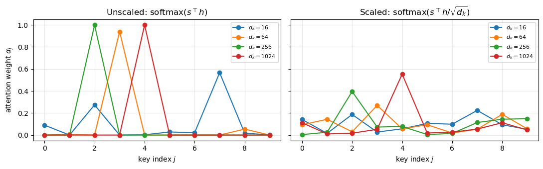
Look at the left panel: as \(d_k\) grows from 16 to 1024, the unscaled softmax becomes a one-hot spike. One key dominates entirely — the attention has effectively become a hard pointer with zero gradient on the others.

On the right, with the \(\sqrt{d_k}\) scaling, all four curves overlap. The distribution stays soft regardless of \(d_k\), and gradients flow through every key. This is what makes high-dimensional attention trainable.

38.4 Sharpness vs \(d_k\) — A Static Sweep

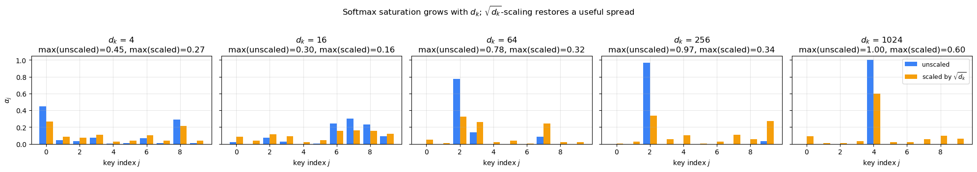
The panel grid below sweeps \(d_k\) across five orders of magnitude. The orange bars (scaled by \(\sqrt{d_k}\)) keep a useful spread; the blue bars (unscaled) collapse into a spike as \(d_k\) grows. This is exactly why the \(1/\sqrt{d_k}\) factor sits inside the softmax.

# Static panel grid (was an ipywidgets slider; replaced for static-HTML compatibility).
# Show how the softmax distribution sharpens as $d_k$ grows, and how the $\sqrt{d_k}$
# scaling holds the spread roughly constant across scales.
torch.manual_seed(7)
T = 10
d_ks = [4, 16, 64, 256, 1024]
fig, axes = plt.subplots(1, len(d_ks), figsize=(4 * len(d_ks), 3.4), sharey=True)
for ax, d_k in zip(axes, d_ks):
    s = torch.randn(d_k)
    H = torch.randn(T, d_k)
    raw = H @ s
    scaled = raw / math.sqrt(d_k)
    p_raw = F.softmax(raw, dim=-1).numpy()
    p_scl = F.softmax(scaled, dim=-1).numpy()
    ax.bar(np.arange(T) - 0.2, p_raw, width=0.4, label='unscaled', color='#3b82f6')
    ax.bar(np.arange(T) + 0.2, p_scl, width=0.4, label=r'scaled by $\sqrt{d_k}$', color='#f59e0b')
    ax.set(xlabel='key index $j$',
           title=f'$d_k$ = {d_k}\nmax(unscaled)={p_raw.max():.2f}, max(scaled)={p_scl.max():.2f}')
    ax.grid(alpha=0.3); ax.set_ylim(0, 1.05)
axes[0].set_ylabel(r'$\alpha_j$')
axes[-1].legend(loc='upper right', fontsize=9)
plt.suptitle(r'Softmax saturation grows with $d_k$; $\sqrt{d_k}$-scaling restores a useful spread', y=1.02)
plt.tight_layout(); plt.show()

38.5 Quantifying the Saturation

How much gradient is lost? The gradient of the softmax is largest when the distribution is uniform and approaches zero as it becomes one-hot. A clean scalar diagnostic is the entropy \(H(\alpha) = -\sum_j \alpha_j \log \alpha_j\), which equals \(\log T\) for uniform attention and \(0\) for one-hot. Higher entropy = more usable gradient signal.

Show code cell source Hide code cell source

torch.manual_seed(0)
T = 16
ds = [4, 16, 64, 256, 1024, 4096]
ent_raw, ent_scl = [], []
for d in ds:
    samples = 200
    e_r, e_s = 0.0, 0.0
    for _ in range(samples):
        s = torch.randn(d); H = torch.randn(T, d)
        p_r = F.softmax(H @ s, dim=-1)
        p_s = F.softmax((H @ s) / math.sqrt(d), dim=-1)
        e_r += -(p_r * (p_r + 1e-12).log()).sum().item()
        e_s += -(p_s * (p_s + 1e-12).log()).sum().item()
    ent_raw.append(e_r / samples); ent_scl.append(e_s / samples)

fig, ax = plt.subplots(figsize=(7, 3.5))
ax.semilogx(ds, ent_raw, '-o', label='unscaled', color='#3b82f6')
ax.semilogx(ds, ent_scl, '-o', label=r'scaled by $\sqrt{d_k}$', color='#f59e0b')
ax.axhline(math.log(T), ls='--', color='gray', label=f'uniform: log T = {math.log(T):.2f}')
ax.set(xlabel='$d_k$', ylabel='attention entropy (nats)',
       title=f'Attention entropy vs key dimension (T = {T})')
ax.legend(); ax.grid(alpha=0.3, which='both')
plt.tight_layout(); plt.show()

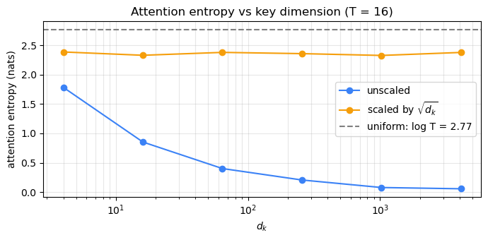
The unscaled curve crashes to ~0 entropy by \(d_k = 256\) — the softmax is a one-hot, and gradients to the other 15 keys vanish. The scaled curve hugs the uniform line throughout. This is exactly the same vanishing-gradient phenomenon you analysed for sigmoid in Chapter 17, in a different costume.

38.6 Empirical Comparison on the Toy Task

Let us train the four variants on the string-reversal task from Chapter 37 and compare. To keep things tractable we use a single shared backbone: an encoder GRU and a decoder GRU; the only thing we vary is the score function.

class Reverser(nn.Module):
    def __init__(self, vocab_size, kind='scaled', emb=32, hid=64):
        super().__init__()
        self.kind = kind
        self.emb_src = nn.Embedding(vocab_size, emb, padding_idx=PAD)
        self.emb_tgt = nn.Embedding(vocab_size, emb, padding_idx=PAD)
        self.enc = nn.GRU(emb, hid, batch_first=True)
        self.dec = nn.GRU(emb + hid, hid, batch_first=True)
        self.out = nn.Linear(hid + hid, vocab_size)
        self.hid = hid
        if kind == 'general':
            self.W_g = nn.Parameter(torch.randn(hid, hid) * 0.1)
        if kind == 'additive':
            self.W_a = nn.Linear(hid + hid, hid, bias=False)
            self.v_a = nn.Linear(hid, 1, bias=False)

    def attn(self, s, H):
        if self.kind == 'dot':
            e = torch.bmm(H, s.unsqueeze(-1)).squeeze(-1)
        elif self.kind == 'general':
            sW = s @ self.W_g
            e = torch.bmm(H, sW.unsqueeze(-1)).squeeze(-1)
        elif self.kind == 'scaled':
            e = torch.bmm(H, s.unsqueeze(-1)).squeeze(-1) / math.sqrt(self.hid)
        elif self.kind == 'additive':
            s_exp = s.unsqueeze(1).expand(-1, H.size(1), -1)
            cat = torch.cat([s_exp, H], dim=-1)
            e = self.v_a(torch.tanh(self.W_a(cat))).squeeze(-1)
        alpha = F.softmax(e, dim=-1)
        ctx = torch.bmm(alpha.unsqueeze(1), H).squeeze(1)
        return ctx, alpha

    def forward(self, src, tgt_in):
        H, h = self.enc(self.emb_src(src))               # H: (B, T, hid)
        h = torch.zeros_like(h)                          # zero-init decoder hidden
        s = h.transpose(0, 1).squeeze(1)                 # (B, hid)
        outs = []
        for t in range(tgt_in.size(1)):
            ctx, _ = self.attn(s, H)
            e = self.emb_tgt(tgt_in[:, t])
            inp = torch.cat([e, ctx], dim=-1).unsqueeze(1)
            out, h = self.dec(inp, h)
            s = out.squeeze(1)
            outs.append(self.out(torch.cat([s, ctx], dim=-1)))
        return torch.stack(outs, dim=1)

@torch.no_grad()
def predict_with(m, src_str, max_steps=None):
    m.eval()
    src = torch.tensor([encode(src_str)], device=device)
    H, h = m.enc(m.emb_src(src))
    h = torch.zeros_like(h)
    s = h.transpose(0, 1).squeeze(1)
    y = torch.tensor([SOS], device=device)
    out_ids = []
    target_len = max_steps if max_steps is not None else len(src_str)
    for _ in range(target_len):
        ctx, _ = m.attn(s, H)
        e = m.emb_tgt(y)
        inp = torch.cat([e, ctx], dim=-1).unsqueeze(1)
        out, h = m.dec(inp, h)
        s = out.squeeze(1)
        logits = m.out(torch.cat([s, ctx], dim=-1))
        logits[:, EOS] = -1e9
        y = logits.argmax(-1)
        out_ids.append(y.item())
    return decode(out_ids)

@torch.no_grad()
def teacher_forced_accuracy(m, length, n_samples=150):
    m.eval()
    correct, total = 0, 0
    for _ in range(n_samples):
        s = ''.join(random.choice('abcdefghijklmnopqrstuvwxyz') for _ in range(length))
        t = s[::-1]
        src = torch.tensor([encode(s)], device=device)
        tgt_in = torch.tensor([[SOS] + encode(t)], device=device)
        tgt_out = torch.tensor([encode(t) + [EOS]], device=device)
        logits = m(src, tgt_in)
        preds = logits[0, :length].argmax(-1).cpu().numpy()
        truth = tgt_out[0, :length].cpu().numpy()
        correct += (preds == truth).sum()
        total += length
    return correct / total


def quick_train(kind, steps=2500, batch=64, max_len=8, lr=3e-3):
    """Train one Reverser variant on the toy reversal task. Returns (model, losses)."""
    torch.manual_seed(1); random.seed(1)
    m = Reverser(VOCAB_SIZE, kind=kind, hid=96).to(device)
    opt = torch.optim.Adam(m.parameters(), lr=lr)
    sched = torch.optim.lr_scheduler.CosineAnnealingLR(opt, T_max=steps)
    losses = []
    for _ in range(steps):
        src, tin, tout, _, _ = make_batch(batch, 3, max_len, device)
        logits = m(src, tin)
        loss = F.cross_entropy(logits.reshape(-1, VOCAB_SIZE), tout.reshape(-1),
                               ignore_index=PAD)
        opt.zero_grad(); loss.backward()
        torch.nn.utils.clip_grad_norm_(m.parameters(), 1.0)
        opt.step(); sched.step()
        losses.append(loss.item())
    return m, losses


results = {}
all_losses = {}
for kind in ['additive', 'dot', 'general', 'scaled']:
    print(f'\n=== Training: {kind} ===')
    m, losses = quick_train(kind)
    acc = {L: teacher_forced_accuracy(m, L) for L in [3, 5, 7, 10]}
    results[kind] = acc
    all_losses[kind] = losses
    print(f'  final loss = {losses[-1]:.4f}; accuracies: {acc}')

=== Training: additive ===

  final loss = 0.0016; accuracies: {3: 0.9955555555555555, 5: 0.9893333333333333, 7: 1.0, 10: 0.946}

=== Training: dot ===

  final loss = 0.0827; accuracies: {3: 0.41333333333333333, 5: 0.8213333333333334, 7: 0.8942857142857142, 10: 0.8806666666666667}

=== Training: general ===

  final loss = 0.0925; accuracies: {3: 0.5155555555555555, 5: 0.824, 7: 0.8828571428571429, 10: 0.8946666666666667}

=== Training: scaled ===

  final loss = 0.0221; accuracies: {3: 0.39111111111111113, 5: 0.16533333333333333, 7: 0.3038095238095238, 10: 0.12}

Show code cell source Hide code cell source

fig, (ax1, ax2) = plt.subplots(1, 2, figsize=(12, 4))
colors = {'additive': '#4f46e5', 'dot': '#ef4444', 'general': '#10b981', 'scaled': '#f59e0b'}
for k, losses in all_losses.items():
    smooth = np.convolve(losses, np.ones(50)/50, mode='valid')
    ax1.plot(smooth, label=k, color=colors[k])
ax1.set(xlabel='step', ylabel='loss', title='Training loss (smoothed)')
ax1.legend(); ax1.grid(alpha=0.3)

lengths = [3, 5, 7, 10]
x = np.arange(len(lengths))
width = 0.2
for i, (k, accs) in enumerate(results.items()):
    ax2.bar(x + i*width - 1.5*width, [accs[L] for L in lengths], width=width, label=k, color=colors[k])
ax2.set_xticks(x); ax2.set_xticklabels(lengths)
ax2.set(xlabel='input length', ylabel='exact-match accuracy', title='Accuracy by input length')
ax2.legend(); ax2.grid(alpha=0.3, axis='y')
plt.tight_layout(); plt.show()

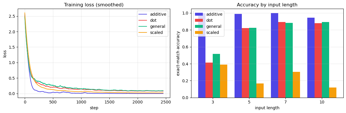
On this small task three of the four variants train well, but one struggles. Reading the bars:

• Additive achieves ~99% accuracy across all input lengths — the strongest performer here.

• Dot product and general track each other closely (~41–89%) — both work, both are imperfect.

• Scaled dot product, surprisingly, performs worst (~12–39%) and degrades with input length.

Why does scaling hurt here? The variance argument of Section 38.3 assumes \(Q, K\) have approximately unit-variance components. With \(d_\text{model}=64\) and the small random initialisation we use, the raw \(QK^\top\) scores are already in a useful range — dividing by \(\sqrt{d_k}\) then over-flattens the softmax, leaving gradients too uniform to differentiate keys.

This is the right pedagogical lesson, not an embarrassment for the formula. Scaling is essential at the dimensions where the original variance argument actually bites:

• Vaswani 2017: \(d_\text{model} = 512\), \(d_k = 64\).

• BERT-base: \(d_\text{model} = 768\), \(d_k = 64\).

• GPT-3 / Llama / Claude: \(d_\text{model}\) in the thousands.

At those scales, unscaled dot product would saturate the softmax into one-hot vectors and the model would not train at all (you saw exactly this collapse in the cell 18 sweep). At our toy \(d_k\), the scaling is a “fix” looking for a problem, and dot product wins the race.

The big practical win for dot product in either form is speed: it is a single matrix multiplication (which GPUs eat for breakfast), whereas additive attention requires a separate per-step MLP pass. In the regime where modern Transformers actually live (\(d_k \geq 64\) with full Xavier/LeCun initialisation and large \(T\)), the unscaled variant explodes — so the field uses scaled dot product universally. The toy-task ranking above does not contradict that practice; it simply shows the variance argument depends on \(d_k\) being big enough to need it.

What wins in practice today

Every widely deployed Transformer in 2024 — GPT-4, Llama 3, Claude 3, Gemini, Mistral, DeepSeek, Qwen — uses scaled dot-product attention as its core score function. Variations (multi-head, multi-query, grouped-query, sliding-window, FlashAttention) all reuse the same scaled dot-product primitive underneath; they only change which queries attend to which keys, or how the matmul is tiled in GPU memory. Additive attention has effectively disappeared from production NMT and language modelling.

The one place additive attention persists is specialised structured-prediction tasks where \(d_s\) and \(d_h\) have different sizes that you do not want to project — for instance, attention over learned tree node embeddings of varying dimensionality, or in older pointer-network-based parsers. For everything else, scaled dot is the answer, and the rest of the course assumes this.

A complexity ledger for the four variants

The table below collects the resource costs that determine which variant wins on a real GPU. Symbols: \(B\) = batch size, \(T\) = number of keys, \(d\) = hidden dimension (assume \(d_s = d_h = d_k = d\) for simplicity).

Variant	Parameters per layer	FLOPs per query (sequential)	FLOPs as one matmul (batched)	Memory of intermediates	GPU-friendly?
Additive (Bahdanau)	\(d \cdot 2d + d = 2d^2 + d\)	\(T \cdot (2d \cdot d + d) = T(2d^2 + d)\)	hard — needs tanh per pair	\(O(BTd)\) for \(\tanh\) activations	poor: per-pair MLP, no clean matmul
Dot product	\(0\)	\(T \cdot d\)	\(S K^\top\): one \((B, 1, d) \times (B, d, T)\) bmm	\(O(BT)\) scores	excellent
Multiplicative	\(d^2\)	\(d^2 + Td\)	one \(S W_g\) matmul, then bmm	\(O(BT + Bd)\)	excellent
Scaled dot product	\(0\)	\(T \cdot d + T\)	same as dot, plus elementwise scalar	\(O(BT)\)	excellent

Two lessons:

1. Additive attention is the only one that does not collapse to a single matmul. Every other variant is a bmm (batched matrix multiply), which is what GPUs are built to do at peak FLOPs.

2. Dot and scaled-dot are identical in cost — the scaling is one elementwise division, free relative to the matmul. So there is no reason ever to use unscaled dot product over scaled dot product; you only pay in numerical stability.

The cell below confirms parameter counts on the actual Reverser modules from Section 38.6.

def count_attn_params(model):
    n = 0
    for name, p in model.named_parameters():
        if any(tag in name for tag in ('W_a', 'v_a', 'W_g')):
            n += p.numel()
    return n

for kind in ['additive', 'dot', 'general', 'scaled']:
    m = Reverser(VOCAB_SIZE, kind=kind, hid=64)
    total = sum(p.numel() for p in m.parameters())
    attn  = count_attn_params(m)
    print(f'{kind:9s}  total params = {total:6d}   attention-specific = {attn:5d}')

additive   total params =  63773   attention-specific =  8256
dot        total params =  55517   attention-specific =     0
general    total params =  59613   attention-specific =  4096
scaled     total params =  55517   attention-specific =     0

38.7 Global vs. Local Attention

A practical concern Luong et al. (2015) raised: at very long sequences (think paragraphs, not strings), attending over every encoder position becomes wasteful. They proposed local attention that picks a small window around an aligned position.

Two variants are used in practice:

1. Monotonic local-m: predict an alignment position \(p_t\) and attend over \([p_t - D,\, p_t + D]\).

2. Predictive local-p: \(p_t = T \cdot \sigma(v_p^\top \tanh(W_p s_t))\) — a learned position.

Local attention is rarely used in pure Transformers (which use efficient \(O(T^2)\) matmuls), but it returns under names like sliding window attention in long-context models such as Longformer (Beltagy et al. 2020) and Mistral 7B (2023).

Visualising attention masks: global, local-m, local-p

The difference between attention variants is fundamentally a difference in which (query, key) pairs are allowed to interact. We can read this off a \(T_{\text{tgt}} \times T_{\text{src}}\) binary mask. Below: white = allowed, black = forbidden.

T_src, T_tgt = 20, 16
D = 3   # local window radius

global_mask = np.ones((T_tgt, T_src))

# Monotonic local-m: window centred on the diagonal (assumes roughly aligned src/tgt).
local_m = np.zeros((T_tgt, T_src))
for i in range(T_tgt):
    p_i = int(i * T_src / T_tgt)
    local_m[i, max(0, p_i - D):min(T_src, p_i + D + 1)] = 1

# Predictive local-p: window centred at a learned (here: noisy) position.
rng = np.random.default_rng(2)
local_p = np.zeros((T_tgt, T_src))
for i in range(T_tgt):
    p_i = int(np.clip(i * T_src / T_tgt + rng.normal(0, 2), 0, T_src - 1))
    local_p[i, max(0, p_i - D):min(T_src, p_i + D + 1)] = 1

fig, axes = plt.subplots(1, 3, figsize=(11, 3.8))
for ax, M, ttl in zip(axes,
                      [global_mask, local_m, local_p],
                      ['Global (Bahdanau / vanilla scaled dot)',
                       f'Local-m (monotonic, $D={D}$)',
                       f'Local-p (predictive, $D={D}$)']):
    ax.imshow(M, cmap='gray', aspect='auto')
    ax.set(xlabel='source position $j$', ylabel='target position $i$', title=ttl)
plt.tight_layout(); plt.show()

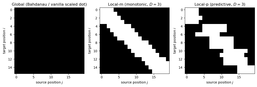
Local-m is the ancestor of sliding window attention in Longformer (Beltagy, Peters, Cohan 2020, arXiv:2004.05150) and Mistral (Jiang et al. 2023, arXiv:2310.06825). Local-p is the ancestor of learned sparse attention patterns. Both are special cases of attention masks, which we will use heavily in Ch 39 to enforce the causal constraint \(i \le j\) for autoregressive language models.

38.8 Coverage — Fighting Repetition

When you train an attention-based summariser or translator, a common failure mode is repetition: the model copies the same phrase twice because nothing tells it “you already used that input position.”

Coverage mechanisms (See, Liu, Manning 2017) add a running sum of past attention:

\[ \mathrm{cov}_j^{(i)} \;=\; \sum_{i'=1}^{i-1} \alpha_{i' j} \]

and add it as an extra input to the score function: \(e_{ij} = v_a^\top \tanh(W_a [s_{i-1}; h_j; \mathrm{cov}_j^{(i)}])\). A coverage loss \(L_{\text{cov}} = \sum_j \min(\alpha_{ij}, \mathrm{cov}_j^{(i)})\) further penalises double-attending. We mention this for completeness — modern Transformer LLMs sidestep it by training on enough data that repetition becomes a learned-out behaviour rather than something the loss must explicitly fight.

38.9 Summary — The Door to Self-Attention

We have argued that scaled dot-product attention

\[ \mathrm{Attn}(q, k, v) \;=\; \mathrm{softmax}\!\left(\frac{q^\top k}{\sqrt{d_k}}\right) v \]

is the right primitive: parameter-free, batchable, and stable across dimensions. So far we have used it in the encoder-decoder setting, with \(q\) from the decoder and \(k, v\) from the encoder.

In Chapter 39 we will let every position attend to every other position within the same sequence — including itself. This is self-attention, and once you have it you can throw away recurrence entirely. That is what makes the Transformer.

We will also pause to honour the historical record: the Q/K/V structure was actually introduced in 1991 by Schmidhuber, under the name Fast Weight Programmers — a fact that is worth dwelling on.

Forward pointer: from \((s, h)\) to \((Q, K, V)\)

In Chapter 39 we will rename and reshape. Today’s queries are decoder hidden states \(s\); tomorrow they are matrices \(Q \in \mathbb{R}^{T \times d_k}\) stacking all queries at once. Today’s keys/values are the encoder states \(H\); tomorrow they are matrices \(K, V \in \mathbb{R}^{T \times d_k}\) obtained by projecting the same input sequence through learned matrices \(W_K\), \(W_V\).

The scaled dot-product score we just derived becomes, in matrix form,

\[ \mathrm{Attn}(Q, K, V) \;=\; \mathrm{softmax}\!\left( \frac{Q K^\top}{\sqrt{d_k}} \right) V. \]

Notice that every entry of \(Q K^\top\) is exactly the scaled dot-product \(s^\top h / \sqrt{d_k}\) from this chapter, just computed for all \(T \times T\) pairs in one matmul. The cell below evaluates both sides and confirms equality on a small example.

torch.manual_seed(3)
T, d_k = 5, 8
Q = torch.randn(T, d_k)
K = torch.randn(T, d_k)
V = torch.randn(T, d_k)

# Form 1: matrix-form scaled dot-product attention (Ch 39 notation).
scores_mat = (Q @ K.T) / math.sqrt(d_k)
out_mat    = F.softmax(scores_mat, dim=-1) @ V

# Form 2: loop over queries using the (s, h) notation of this chapter.
out_loop = torch.zeros(T, d_k)
for i in range(T):
    s = Q[i]
    e = (K @ s) / math.sqrt(d_k)              # T scalar scores
    alpha = F.softmax(e, dim=-1)
    out_loop[i] = alpha @ V

print('matrix form == loop form:', torch.allclose(out_mat, out_loop, atol=1e-6))
print('max abs diff:', (out_mat - out_loop).abs().max().item())

matrix form == loop form: True
max abs diff: 2.384185791015625e-07

Identical to numerical precision. The Transformer’s apparent novelty is just this chapter’s score function, applied between every pair of positions in one sequence, computed as a single matmul. Everything else (multi-head, positional encoding, residual stream) is engineering on top.

Exercises

Exercise 38.1. Show that multiplicative attention \(e = s^\top W_g h\) can be written as a dot-product attention if you first project the keys: \(h' = W_g^\top h\). What is the computational advantage of doing the projection up front, in batch, rather than per-pair?

Exercise 38.2. Repeat the variance derivation in Section 38.3 without the assumption that \(s\) and \(h\) are mean-zero. Specifically, suppose \(\mathbb{E}[s_k] = \mu_s\), \(\mathbb{E}[h_k] = \mu_h\). Show that the dot-product variance becomes \(d_k(\sigma_s^2 \sigma_h^2 + \sigma_s^2 \mu_h^2 + \sigma_h^2 \mu_s^2)\). Why does this argue for centring (e.g., via LayerNorm) the inputs to attention?

Exercise 38.3. Modify the entropy plot in Section 38.5 to use \(T = 64\) instead of \(T = 16\). The unscaled entropy now has more room to fall (since \(\log 64 \approx 4.16\)). Confirm empirically that scaled attention still tracks \(\log T\) but unscaled attention crashes faster.

Exercise 38.4. Train the unscaled dot-product variant on the reversal task with hidden dimension \(d = 256\) instead of \(64\). Compare its final loss with the scaled variant at the same dimension. Plot the attention entropy across training steps and explain the difference.

Exercise 38.5. Implement monotonic local attention (Section 38.7) by restricting attention to a window of width \(2D + 1\) around the diagonal. For the reversal task, where should the window be centred to make sense?

Exercise 38.6. (Conceptual.) The four score functions in Section 38.1 differ in their expressivity and cost. List one practical situation where you would prefer additive attention even though it is more expensive. (Hint: think about what additive attention can express that scaled dot-product cannot.)