Chapter 16: Backpropagation – The Complete Derivation#
This chapter is the mathematical centerpiece of the course. We derive the backpropagation algorithm from first principles, establishing the four fundamental equations that enable efficient computation of gradients in multilayer neural networks.
Backpropagation solves the credit assignment problem: given an error at the output, how should each weight in the network be adjusted?
Note
Historical credit – The ideas behind backpropagation have a rich and sometimes contentious history. Key contributors include: Bryson (1961) and Dreyfus (1962) in optimal control, Linnainmaa (1970) who formalized reverse-mode automatic differentiation, Werbos (1974) who first applied it to neural networks in his Harvard PhD thesis, and Rumelhart, Hinton & Williams (1986) whose Nature paper popularized the algorithm and demonstrated its power for learning internal representations.
16.1 Network Architecture and Notation#
Consider a feedforward neural network with \(L\) layers.
Notation#
Symbol |
Meaning |
|---|---|
\(L\) |
Number of layers (not counting input) |
\(n_l\) |
Number of neurons in layer \(l\) |
\(\mathbf{W}^{(l)} \in \mathbb{R}^{n_l \times n_{l-1}}\) |
Weight matrix for layer \(l\) |
\(\mathbf{b}^{(l)} \in \mathbb{R}^{n_l}\) |
Bias vector for layer \(l\) |
\(\mathbf{z}^{(l)} \in \mathbb{R}^{n_l}\) |
Pre-activation (weighted input) for layer \(l\) |
\(\mathbf{a}^{(l)} \in \mathbb{R}^{n_l}\) |
Post-activation (output) of layer \(l\) |
\(\sigma^{(l)}\) |
Activation function for layer \(l\) |
\(\mathbf{a}^{(0)} = \mathbf{x}\) |
Input to the network |
Forward Pass#
For each layer \(l = 1, 2, \ldots, L\):
The network output is \(\hat{\mathbf{y}} = \mathbf{a}^{(L)}\).
The loss for a single training example is \(\mathcal{L} = L(\mathbf{a}^{(L)}, \mathbf{y})\).
16.2 The Chain Rule of Calculus#
Univariate Chain Rule – Full Proof#
Theorem (Chain Rule)
Let \(f\) and \(g\) be differentiable functions. If \(h(x) = f(g(x))\), then:
Equivalently, if \(y = f(u)\) and \(u = g(x)\), then \(\frac{dy}{dx} = \frac{dy}{du} \cdot \frac{du}{dx}\).
This is the mathematical engine that drives backpropagation: to compute how the loss depends on early-layer parameters, we chain together derivatives through all intermediate computations.
Proof
Let \(u = g(x)\). We want to show \(\frac{dh}{dx} = \frac{df}{du} \cdot \frac{du}{dx}\).
By definition:
Let \(\Delta u = g(x + \Delta x) - g(x)\). Note that \(\Delta u \to 0\) as \(\Delta x \to 0\) (since \(g\) is continuous, being differentiable).
Case 1: If \(\Delta u \neq 0\) for all sufficiently small \(\Delta x\):
Case 2 (General): Define the auxiliary function:
Note that \(\lim_{\Delta u \to 0} \phi(\Delta u) = 0\) (by differentiability of \(f\)), so \(\phi\) is continuous at 0.
We can write:
This holds for all \(\Delta u\) (including \(\Delta u = 0\)). Therefore:
Taking the limit as \(\Delta x \to 0\): since \(\Delta u \to 0\), we have \(\phi(\Delta u) \to 0\), and \(\Delta u / \Delta x \to g'(x)\). Thus:
Multivariate Chain Rule#
For \(\mathbf{z} = f(\mathbf{u})\) and \(\mathbf{u} = g(\mathbf{x})\), the chain rule gives:
In Jacobian notation: \(\mathbf{J}_{\mathbf{z}/\mathbf{x}} = \mathbf{J}_{\mathbf{z}/\mathbf{u}} \cdot \mathbf{J}_{\mathbf{u}/\mathbf{x}}\).
This matrix formulation is the key to understanding backpropagation: the gradient propagates backward through the network as a product of Jacobians.
16.3 The Error Signal#
Definition. The error signal (or local gradient) for neuron \(j\) in layer \(l\) is:
This measures how sensitive the loss is to changes in the pre-activation of that neuron.
In vector form: \(\boldsymbol{\delta}^{(l)} = \nabla_{\mathbf{z}^{(l)}} \mathcal{L}\).
The error signal is the central quantity in backpropagation. Once we know \(\boldsymbol{\delta}^{(l)}\) for each layer, computing all gradients becomes straightforward.
16.4 The Four Fundamental Equations of Backpropagation#
Equation (BP1 – Output Layer Error)
The error signal at the output layer is the element-wise product of the loss gradient with respect to the output activations and the derivative of the activation function evaluated at the pre-activations.
Example (MSE loss): \(\nabla_{\mathbf{a}^{(L)}} \mathcal{L} = \mathbf{a}^{(L)} - \mathbf{y}\), so \(\boldsymbol{\delta}^{(L)} = (\mathbf{a}^{(L)} - \mathbf{y}) \odot \sigma'^{(L)}(\mathbf{z}^{(L)})\).
Derivation. By the chain rule:
Since \(a_k^{(L)} = \sigma^{(L)}(z_k^{(L)})\) and activation functions are applied element-wise:
Therefore:
In vector form with \(\odot\) denoting element-wise multiplication: \(\boldsymbol{\delta}^{(L)} = \nabla_{\mathbf{a}^{(L)}} \mathcal{L} \odot \sigma'^{(L)}(\mathbf{z}^{(L)})\). \(\blacksquare\)
Equation (BP2 – Error Backpropagation)
The error at layer \(l\) is computed from the error at layer \(l+1\) by multiplying by the transpose of the weight matrix (“back” propagation) and element-wise multiplying with the activation derivative. This is the recursive equation that gives the algorithm its name.
Derivation. For layer \(l < L\), apply the chain rule through layer \(l+1\):
Now compute \(\frac{\partial z_k^{(l+1)}}{\partial z_j^{(l)}}\). Since \(z_k^{(l+1)} = \sum_m W_{km}^{(l+1)} a_m^{(l)} + b_k^{(l+1)}\) and \(a_m^{(l)} = \sigma^{(l)}(z_m^{(l)})\):
Substituting:
In vector form: \(\boldsymbol{\delta}^{(l)} = ((\mathbf{W}^{(l+1)})^\top \boldsymbol{\delta}^{(l+1)}) \odot \sigma'^{(l)}(\mathbf{z}^{(l)})\). \(\blacksquare\)
Key insight: The error at layer \(l\) is computed from the error at layer \(l+1\) by multiplying by the transpose of the weight matrix. This is why the algorithm is called “back” propagation – errors flow backward through the network.
Equation (BP3 – Weight Gradients)
The gradient of the loss with respect to a weight matrix is the outer product of the error signal at the output side and the activation at the input side of that weight. This has a “Hebbian” structure – modulated by the error signal.
Derivation. Since \(z_j^{(l)} = \sum_k W_{jk}^{(l)} a_k^{(l-1)} + b_j^{(l)}\):
In matrix form: \(\frac{\partial \mathcal{L}}{\partial \mathbf{W}^{(l)}} = \boldsymbol{\delta}^{(l)} (\mathbf{a}^{(l-1)})^\top\). \(\blacksquare\)
Equation (BP4 – Bias Gradients)
The gradient with respect to the bias is simply the error signal itself. The bias has a direct, unscaled influence on the pre-activation \(z_j^{(l)}\).
Derivation. Since \(z_j^{(l)} = \sum_k W_{jk}^{(l)} a_k^{(l-1)} + b_j^{(l)}\):
Danger
❗ Numerical instability in deep networks – Gradients can explode or vanish when propagated through many layers. From BP2, the error signal is a product of \((L - l)\) terms, each involving \(\sigma'\) and a weight matrix. If these factors are consistently \(< 1\), gradients vanish exponentially; if consistently \(> 1\), they explode. This is why deep networks were impractical until ~2010, when solutions like ReLU, careful initialization, and batch normalization were developed.
Tip
Computational efficiency – The backward pass has the SAME time complexity as the forward pass, \(O(L \cdot n^2)\) for a network with \(L\) layers of width \(n\). Computing all gradients via backpropagation costs only about twice the forward pass. This is vastly more efficient than numerical finite differences, which require about \(P\) additional forward evaluations for a one-sided check, or about \(2P\) for centered differences, where \(P\) is the total number of parameters.
16.5 Worked Numerical Example#
Consider a network with:
Input layer: 2 neurons (\(n_0 = 2\))
Hidden layer: 3 neurons (\(n_1 = 3\)), sigmoid activation
Output layer: 1 neuron (\(n_2 = 1\)), sigmoid activation
Loss: MSE, \(\mathcal{L} = \frac{1}{2}(a^{(2)} - y)^2\)
Specific Weights#
Input: \(\mathbf{x} = (0.05, 0.10)^\top\), Target: \(y = 0.01\)
Show code cell source
import numpy as np

# ============================================================
# Worked Numerical Example: Complete Forward and Backward Pass
# ============================================================

def sigmoid(z):
    return 1 / (1 + np.exp(-z))

def sigmoid_derivative(z):
    s = sigmoid(z)
    return s * (1 - s)

# Network parameters
W1 = np.array([[0.15, 0.20],
               [0.25, 0.30],
               [0.35, 0.40]])
b1 = np.array([[0.35], [0.35], [0.35]])

W2 = np.array([[0.40, 0.45, 0.50]])
b2 = np.array([[0.60]])

# Input and target
x = np.array([[0.05], [0.10]])  # 2x1
y = np.array([[0.01]])           # 1x1

print("="*60)
print("FORWARD PASS")
print("="*60)

# Layer 1
z1 = W1 @ x + b1
a1 = sigmoid(z1)

print(f"\nLayer 1 pre-activation z^(1):")
for i in range(3):
    terms = " + ".join([f"{W1[i,j]:.2f}*{x[j,0]:.2f}" for j in range(2)])
    print(f"  z^(1)_{i+1} = {terms} + {b1[i,0]:.2f} = {z1[i,0]:.6f}")

print(f"\nLayer 1 activation a^(1) = sigma(z^(1)):")
for i in range(3):
    print(f"  a^(1)_{i+1} = sigma({z1[i,0]:.6f}) = {a1[i,0]:.6f}")

# Layer 2
z2 = W2 @ a1 + b2
a2 = sigmoid(z2)

print(f"\nLayer 2 pre-activation z^(2):")
terms = " + ".join([f"{W2[0,j]:.2f}*{a1[j,0]:.6f}" for j in range(3)])
print(f"  z^(2)_1 = {terms} + {b2[0,0]:.2f}")
print(f"         = {z2[0,0]:.6f}")

print(f"\nOutput: a^(2) = sigma({z2[0,0]:.6f}) = {a2[0,0]:.6f}")
print(f"Target: y = {y[0,0]}")

# Loss
loss = 0.5 * (a2[0,0] - y[0,0])**2
print(f"\nLoss: L = 0.5 * ({a2[0,0]:.6f} - {y[0,0]})^2 = {loss:.6f}")

print("\n" + "="*60)
print("BACKWARD PASS")
print("="*60)

# BP1: Output layer error
dL_da2 = a2 - y  # gradient of MSE w.r.t. output activation
sigma_prime_z2 = sigmoid_derivative(z2)
delta2 = dL_da2 * sigma_prime_z2

print(f"\n--- BP1: Output layer error ---")
print(f"  dL/da^(2) = a^(2) - y = {a2[0,0]:.6f} - {y[0,0]} = {dL_da2[0,0]:.6f}")
print(f"  sigma'(z^(2)) = sigma(z^(2)) * (1 - sigma(z^(2))) = {a2[0,0]:.6f} * {1-a2[0,0]:.6f} = {sigma_prime_z2[0,0]:.6f}")
print(f"  delta^(2) = {dL_da2[0,0]:.6f} * {sigma_prime_z2[0,0]:.6f} = {delta2[0,0]:.6f}")

# BP2: Hidden layer error
delta1 = (W2.T @ delta2) * sigmoid_derivative(z1)

print(f"\n--- BP2: Hidden layer error ---")
print(f"  (W^(2))^T * delta^(2):")
W2T_delta2 = W2.T @ delta2
for i in range(3):
    print(f"    [{W2[0,i]:.2f}] * {delta2[0,0]:.6f} = {W2T_delta2[i,0]:.6f}")
print(f"  sigma'(z^(1)):")
sp1 = sigmoid_derivative(z1)
for i in range(3):
    print(f"    sigma'({z1[i,0]:.6f}) = {sp1[i,0]:.6f}")
print(f"  delta^(1) = (W^T delta^(2)) * sigma'(z^(1)):")
for i in range(3):
    print(f"    delta^(1)_{i+1} = {W2T_delta2[i,0]:.6f} * {sp1[i,0]:.6f} = {delta1[i,0]:.6f}")

# BP3: Weight gradients
dL_dW2 = delta2 @ a1.T
dL_dW1 = delta1 @ x.T

print(f"\n--- BP3: Weight gradients ---")
print(f"  dL/dW^(2) = delta^(2) * (a^(1))^T:")
for j in range(3):
    print(f"    dL/dW^(2)_{{1,{j+1}}} = {delta2[0,0]:.6f} * {a1[j,0]:.6f} = {dL_dW2[0,j]:.6f}")
print(f"  dL/dW^(1) = delta^(1) * x^T:")
for i in range(3):
    for j in range(2):
        print(f"    dL/dW^(1)_{{{i+1},{j+1}}} = {delta1[i,0]:.6f} * {x[j,0]:.2f} = {dL_dW1[i,j]:.8f}")

# BP4: Bias gradients
dL_db2 = delta2
dL_db1 = delta1

print(f"\n--- BP4: Bias gradients ---")
print(f"  dL/db^(2) = delta^(2) = {dL_db2[0,0]:.6f}")
for i in range(3):
    print(f"  dL/db^(1)_{i+1} = delta^(1)_{i+1} = {dL_db1[i,0]:.6f}")

# Update weights (one step)
eta = 0.5
W2_new = W2 - eta * dL_dW2
b2_new = b2 - eta * dL_db2
W1_new = W1 - eta * dL_dW1
b1_new = b1 - eta * dL_db1

print(f"\n--- Updated weights (eta = {eta}) ---")
print(f"  W^(2) new: {W2_new}")
print(f"  W^(1) new:\n{W1_new}")

# Verify with one more forward pass
z1_new = W1_new @ x + b1_new
a1_new = sigmoid(z1_new)
z2_new = W2_new @ a1_new + b2_new
a2_new = sigmoid(z2_new)
loss_new = 0.5 * (a2_new[0,0] - y[0,0])**2
print(f"\nNew output: {a2_new[0,0]:.6f} (was {a2[0,0]:.6f})")
print(f"New loss: {loss_new:.6f} (was {loss:.6f})")
print(f"Loss decreased: {loss_new < loss}")
============================================================
FORWARD PASS
============================================================

Layer 1 pre-activation z^(1):
  z^(1)_1 = 0.15*0.05 + 0.20*0.10 + 0.35 = 0.377500
  z^(1)_2 = 0.25*0.05 + 0.30*0.10 + 0.35 = 0.392500
  z^(1)_3 = 0.35*0.05 + 0.40*0.10 + 0.35 = 0.407500

Layer 1 activation a^(1) = sigma(z^(1)):
  a^(1)_1 = sigma(0.377500) = 0.593270
  a^(1)_2 = sigma(0.392500) = 0.596884
  a^(1)_3 = sigma(0.407500) = 0.600488

Layer 2 pre-activation z^(2):
  z^(2)_1 = 0.40*0.593270 + 0.45*0.596884 + 0.50*0.600488 + 0.60
         = 1.406150

Output: a^(2) = sigma(1.406150) = 0.803158
Target: y = 0.01

Loss: L = 0.5 * (0.803158 - 0.01)^2 = 0.314550

============================================================
BACKWARD PASS
============================================================

--- BP1: Output layer error ---
  dL/da^(2) = a^(2) - y = 0.803158 - 0.01 = 0.793158
  sigma'(z^(2)) = sigma(z^(2)) * (1 - sigma(z^(2))) = 0.803158 * 0.196842 = 0.158095
  delta^(2) = 0.793158 * 0.158095 = 0.125394

--- BP2: Hidden layer error ---
  (W^(2))^T * delta^(2):
    [0.40] * 0.125394 = 0.050158
    [0.45] * 0.125394 = 0.056428
    [0.50] * 0.125394 = 0.062697
  sigma'(z^(1)):
    sigma'(0.377500) = 0.241301
    sigma'(0.392500) = 0.240613
    sigma'(0.407500) = 0.239902
  delta^(1) = (W^T delta^(2)) * sigma'(z^(1)):
    delta^(1)_1 = 0.050158 * 0.241301 = 0.012103
    delta^(1)_2 = 0.056428 * 0.240613 = 0.013577
    delta^(1)_3 = 0.062697 * 0.239902 = 0.015041

--- BP3: Weight gradients ---
  dL/dW^(2) = delta^(2) * (a^(1))^T:
    dL/dW^(2)_{1,1} = 0.125394 * 0.593270 = 0.074393
    dL/dW^(2)_{1,2} = 0.125394 * 0.596884 = 0.074846
    dL/dW^(2)_{1,3} = 0.125394 * 0.600488 = 0.075298
  dL/dW^(1) = delta^(1) * x^T:
    dL/dW^(1)_{1,1} = 0.012103 * 0.05 = 0.00060516
    dL/dW^(1)_{1,2} = 0.012103 * 0.10 = 0.00121031
    dL/dW^(1)_{2,1} = 0.013577 * 0.05 = 0.00067886
    dL/dW^(1)_{2,2} = 0.013577 * 0.10 = 0.00135772
    dL/dW^(1)_{3,1} = 0.015041 * 0.05 = 0.00075206
    dL/dW^(1)_{3,2} = 0.015041 * 0.10 = 0.00150412

--- BP4: Bias gradients ---
  dL/db^(2) = delta^(2) = 0.125394
  dL/db^(1)_1 = delta^(1)_1 = 0.012103
  dL/db^(1)_2 = delta^(1)_2 = 0.013577
  dL/db^(1)_3 = delta^(1)_3 = 0.015041

--- Updated weights (eta = 0.5) ---
  W^(2) new: [[0.36280361 0.41257699 0.46235104]]
  W^(1) new:
[[0.14969742 0.19939484]
 [0.24966057 0.29932114]
 [0.34962397 0.39924794]]

New output: 0.781491 (was 0.803158)
New loss: 0.297599 (was 0.314550)
Loss decreased: True
16.6 The General L-Layer Backpropagation Algorithm#
Algorithm: Backpropagation#
Input: Training sample \((\mathbf{x}, \mathbf{y})\), network parameters \(\{\mathbf{W}^{(l)}, \mathbf{b}^{(l)}\}_{l=1}^{L}\)
Output: Gradients \(\{\partial \mathcal{L}/\partial \mathbf{W}^{(l)}, \partial \mathcal{L}/\partial \mathbf{b}^{(l)}\}_{l=1}^{L}\)
Step 1: Forward Pass
Set \(\mathbf{a}^{(0)} = \mathbf{x}\)
For \(l = 1, 2, \ldots, L\):
Cache all \(\mathbf{z}^{(l)}\) and \(\mathbf{a}^{(l)}\) for use in the backward pass.
Step 2: Compute Output Error (BP1)
Step 3: Backward Pass (BP2)
For \(l = L-1, L-2, \ldots, 1\):
Step 4: Compute Gradients (BP3, BP4)
For \(l = 1, 2, \ldots, L\):
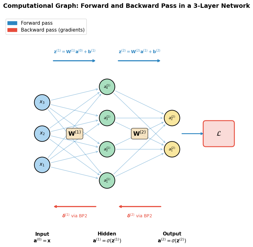
Computational Graph Diagram#
The following code draws a simple 3-layer network as a directed acyclic graph (DAG), showing how data flows forward and gradients flow backward.
Show code cell source
import numpy as np
import matplotlib.pyplot as plt
import matplotlib.patches as mpatches

fig, ax = plt.subplots(figsize=(14, 8))

# Network structure: 3 input, 4 hidden, 2 output
layer_sizes = [3, 4, 2]
layer_names = ['Input\n$\\mathbf{a}^{(0)} = \\mathbf{x}$',
               'Hidden\n$\\mathbf{a}^{(1)} = \\sigma(\\mathbf{z}^{(1)})$',
               'Output\n$\\mathbf{a}^{(2)} = \\sigma(\\mathbf{z}^{(2)})$']
layer_x = [1, 3.5, 6]

node_positions = {}  # (layer, neuron) -> (x, y)

for l, (n, x_pos) in enumerate(zip(layer_sizes, layer_x)):
    y_start = -(n - 1) / 2 * 1.2
    for i in range(n):
        y = y_start + i * 1.2
        node_positions[(l, i)] = (x_pos, y)
        # Draw neuron
        circle = plt.Circle((x_pos, y), 0.3, fill=True,
                           facecolor=['#AED6F1', '#A9DFBF', '#F9E79F'][l],
                           edgecolor='black', linewidth=1.5, zorder=5)
        ax.add_patch(circle)
        # Label
        if l == 0:
            ax.text(x_pos, y, f'$x_{i+1}$', ha='center', va='center', fontsize=11, zorder=6)
        elif l == 1:
            ax.text(x_pos, y, f'$a^{{(1)}}_{i+1}$', ha='center', va='center', fontsize=9, zorder=6)
        else:
            ax.text(x_pos, y, f'$a^{{(2)}}_{i+1}$', ha='center', va='center', fontsize=9, zorder=6)

# Draw forward arrows (blue)
for l in range(len(layer_sizes) - 1):
    for i in range(layer_sizes[l]):
        for j in range(layer_sizes[l + 1]):
            x1, y1 = node_positions[(l, i)]
            x2, y2 = node_positions[(l + 1, j)]
            # Shorten arrows to not overlap circles
            dx = x2 - x1
            dy = y2 - y1
            dist = np.sqrt(dx**2 + dy**2)
            offset = 0.32 / dist
            ax.annotate('', xy=(x2 - dx*offset, y2 - dy*offset),
                       xytext=(x1 + dx*offset, y1 + dy*offset),
                       arrowprops=dict(arrowstyle='->', color='#2E86C1', lw=1.0, alpha=0.5))

# Draw backward arrows (red, below)
for l in range(len(layer_sizes) - 1, 0, -1):
    x_mid = (layer_x[l] + layer_x[l-1]) / 2
    y_bottom = min(v[1] for v in node_positions.values()) - 1.0
    ax.annotate('', xy=(layer_x[l-1] + 0.4, y_bottom),
               xytext=(layer_x[l] - 0.4, y_bottom),
               arrowprops=dict(arrowstyle='->', color='#E74C3C', lw=2.5))
    ax.text(x_mid, y_bottom - 0.35,
            f'$\\boldsymbol{{\\delta}}^{{({l})}}$ via BP2' if l > 1 else '$\\boldsymbol{\\delta}^{(1)}$ via BP2',
            ha='center', va='center', fontsize=10, color='#E74C3C')

# Forward arrow label
y_top = max(v[1] for v in node_positions.values()) + 1.0
for l in range(len(layer_sizes) - 1):
    x_mid = (layer_x[l] + layer_x[l+1]) / 2
    ax.annotate('', xy=(layer_x[l+1] - 0.4, y_top),
               xytext=(layer_x[l] + 0.4, y_top),
               arrowprops=dict(arrowstyle='->', color='#2E86C1', lw=2.5))
    ax.text(x_mid, y_top + 0.35,
            f'$\\mathbf{{z}}^{{({l+1})}} = \\mathbf{{W}}^{{({l+1})}}\\mathbf{{a}}^{{({l})}} + \\mathbf{{b}}^{{({l+1})}}$',
            ha='center', va='center', fontsize=10, color='#2E86C1')

# Layer labels
for l, (name, x_pos) in enumerate(zip(layer_names, layer_x)):
    y_label = min(v[1] for v in node_positions.values()) - 2.2
    ax.text(x_pos, y_label, name, ha='center', va='center', fontsize=11, fontweight='bold')

# Weight labels between layers
for l in range(len(layer_sizes) - 1):
    x_mid = (layer_x[l] + layer_x[l+1]) / 2
    ax.text(x_mid, 0, f'$\\mathbf{{W}}^{{({l+1})}}$', ha='center', va='center',
           fontsize=14, fontweight='bold',
           bbox=dict(boxstyle='round,pad=0.3', facecolor='wheat', alpha=0.8))

# Loss node
loss_x = layer_x[-1] + 1.8
loss_y = 0
rect = mpatches.FancyBboxPatch((loss_x - 0.5, loss_y - 0.4), 1.0, 0.8,
                                boxstyle="round,pad=0.1", facecolor='#FADBD8',
                                edgecolor='#E74C3C', linewidth=2)
ax.add_patch(rect)
ax.text(loss_x, loss_y, '$\\mathcal{L}$', ha='center', va='center', fontsize=16, fontweight='bold')

# Arrow from output to loss
ax.annotate('', xy=(loss_x - 0.55, loss_y),
           xytext=(layer_x[-1] + 0.35, 0),
           arrowprops=dict(arrowstyle='->', color='#2E86C1', lw=2))

# Legend
forward_patch = mpatches.Patch(color='#2E86C1', label='Forward pass')
backward_patch = mpatches.Patch(color='#E74C3C', label='Backward pass (gradients)')
ax.legend(handles=[forward_patch, backward_patch], fontsize=11, loc='upper left')

ax.set_xlim(-0.5, 9)
ax.set_ylim(-4, 4.5)
ax.set_aspect('equal')
ax.axis('off')
ax.set_title('Computational Graph: Forward and Backward Pass in a 3-Layer Network',
             fontsize=14, fontweight='bold', pad=20)

plt.tight_layout()
plt.savefig('computational_graph.png', dpi=150, bbox_inches='tight')
plt.show()
Gradient Flow Visualization#
The following code demonstrates how gradient magnitudes change as they flow backward through a 5-layer network, illustrating potential vanishing/exploding gradient issues.
Show code cell source
import numpy as np
import matplotlib.pyplot as plt

np.random.seed(42)

def sigmoid(z):
    return 1 / (1 + np.exp(-np.clip(z, -500, 500)))

def sigmoid_deriv(z):
    s = sigmoid(z)
    return s * (1 - s)

def relu(z):
    return np.maximum(0, z)

def relu_deriv(z):
    return (z > 0).astype(float)

# 5-layer network: input(10) -> 20 -> 20 -> 20 -> 20 -> 20 -> 1
layer_sizes = [10, 20, 20, 20, 20, 20, 1]
n_layers = len(layer_sizes) - 1

def run_network(activation='sigmoid'):
    """Run forward and backward pass, return gradient norms per layer."""
    # Xavier initialization
    weights = []
    for i in range(n_layers):
        n_in, n_out = layer_sizes[i], layer_sizes[i+1]
        W = np.random.randn(n_out, n_in) * np.sqrt(2.0 / (n_in + n_out))
        weights.append(W)

    # Forward pass
    x = np.random.randn(layer_sizes[0], 1)
    act_fn = sigmoid if activation == 'sigmoid' else relu
    act_deriv = sigmoid_deriv if activation == 'sigmoid' else relu_deriv

    a_list = [x]
    z_list = []
    a = x
    for W in weights:
        z = W @ a
        a = act_fn(z)
        z_list.append(z)
        a_list.append(a)

    # Backward pass
    y = np.random.randn(layer_sizes[-1], 1)
    dL_da = a_list[-1] - y  # MSE gradient
    delta = dL_da * act_deriv(z_list[-1])

    grad_norms = [np.linalg.norm(delta)]

    for l in range(n_layers - 1, 0, -1):
        delta = (weights[l].T @ delta) * act_deriv(z_list[l-1])
        grad_norms.append(np.linalg.norm(delta))

    grad_norms.reverse()
    return grad_norms

# Run for both activations
np.random.seed(42)
sigmoid_grads = run_network('sigmoid')
np.random.seed(42)
relu_grads = run_network('relu')

# Visualize as bar chart and heatmap
fig, axes = plt.subplots(1, 3, figsize=(18, 5))

# Bar chart comparison
x_pos = np.arange(n_layers)
width = 0.35

axes[0].bar(x_pos - width/2, sigmoid_grads, width, label='Sigmoid', color='#E74C3C', alpha=0.8)
axes[0].bar(x_pos + width/2, relu_grads, width, label='ReLU', color='#2ECC71', alpha=0.8)
axes[0].set_xlabel('Layer', fontsize=12)
axes[0].set_ylabel('Gradient Norm $\\|\\boldsymbol{\\delta}^{(l)}\\|$', fontsize=12)
axes[0].set_title('Gradient Magnitude by Layer', fontsize=13)
axes[0].set_xticks(x_pos)
axes[0].set_xticklabels([f'Layer {i+1}' for i in range(n_layers)])
axes[0].set_yscale('log')
axes[0].legend(fontsize=11)
axes[0].grid(True, alpha=0.3, axis='y')

# Heatmap for sigmoid
sigmoid_matrix = np.array(sigmoid_grads).reshape(1, -1)
im1 = axes[1].imshow(np.log10(sigmoid_matrix + 1e-20), aspect='auto', cmap='Reds',
                      vmin=-10, vmax=0)
axes[1].set_xticks(range(n_layers))
axes[1].set_xticklabels([f'L{i+1}' for i in range(n_layers)])
axes[1].set_yticks([])
axes[1].set_title('Sigmoid: Gradient Flow (log scale)', fontsize=13)
axes[1].set_xlabel('Layer', fontsize=12)
for i in range(n_layers):
    axes[1].text(i, 0, f'{sigmoid_grads[i]:.2e}', ha='center', va='center',
                fontsize=8, color='white' if sigmoid_grads[i] < 0.01 else 'black')
plt.colorbar(im1, ax=axes[1], label='log10(gradient norm)')

# Heatmap for ReLU
relu_matrix = np.array(relu_grads).reshape(1, -1)
im2 = axes[2].imshow(np.log10(relu_matrix + 1e-20), aspect='auto', cmap='Greens',
                      vmin=-10, vmax=0)
axes[2].set_xticks(range(n_layers))
axes[2].set_xticklabels([f'L{i+1}' for i in range(n_layers)])
axes[2].set_yticks([])
axes[2].set_title('ReLU: Gradient Flow (log scale)', fontsize=13)
axes[2].set_xlabel('Layer', fontsize=12)
for i in range(n_layers):
    axes[2].text(i, 0, f'{relu_grads[i]:.2e}', ha='center', va='center',
                fontsize=8, color='white' if relu_grads[i] < 0.01 else 'black')
plt.colorbar(im2, ax=axes[2], label='log10(gradient norm)')

plt.suptitle('Gradient Flow in a 6-Layer Network: Sigmoid vs ReLU', fontsize=14, fontweight='bold')
plt.tight_layout()
plt.savefig('gradient_flow.png', dpi=150, bbox_inches='tight')
plt.show()

print("Sigmoid gradient norms (layer 1 to 6):")
for i, g in enumerate(sigmoid_grads):
    print(f"  Layer {i+1}: {g:.6e}")
print(f"  Ratio (layer 1 / layer 6): {sigmoid_grads[0]/sigmoid_grads[-1]:.6e}")
print(f"\nReLU gradient norms (layer 1 to 6):")
for i, g in enumerate(relu_grads):
    print(f"  Layer {i+1}: {g:.6e}")
print(f"  Ratio (layer 1 / layer 6): {relu_grads[0]/relu_grads[-1]:.6e}")
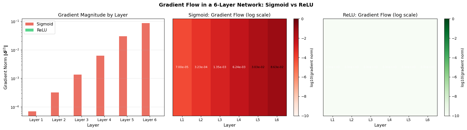
Sigmoid gradient norms (layer 1 to 6):
  Layer 1: 7.002996e-05
  Layer 2: 3.228558e-04
  Layer 3: 1.354784e-03
  Layer 4: 6.242221e-03
  Layer 5: 3.025070e-02
  Layer 6: 8.634400e-02
  Ratio (layer 1 / layer 6): 8.110576e-04

ReLU gradient norms (layer 1 to 6):
  Layer 1: 0.000000e+00
  Layer 2: 0.000000e+00
  Layer 3: 0.000000e+00
  Layer 4: 0.000000e+00
  Layer 5: 0.000000e+00
  Layer 6: 0.000000e+00
  Ratio (layer 1 / layer 6): nan
/var/folders/z7/wp7m8p7x1250jzvklw5z24mm0000gn/T/ipykernel_16506/201685448.py:124: RuntimeWarning: invalid value encountered in scalar divide
  print(f"  Ratio (layer 1 / layer 6): {relu_grads[0]/relu_grads[-1]:.6e}")
16.7 Computational Complexity#
Forward Pass#
The dominant operation in each layer is the matrix-vector product \(\mathbf{W}^{(l)} \mathbf{a}^{(l-1)}\), which costs \(O(n_l \cdot n_{l-1})\).
Total forward pass cost: \(\sum_{l=1}^{L} O(n_l \cdot n_{l-1})\).
For a network with all layers of size \(n\): \(O(L \cdot n^2)\).
Backward Pass#
The dominant operation is \((\mathbf{W}^{(l+1)})^\top \boldsymbol{\delta}^{(l+1)}\), which also costs \(O(n_{l+1} \cdot n_l)\).
Total backward pass cost: \(\sum_{l=1}^{L} O(n_l \cdot n_{l-1})\) – the same order as the forward pass.
Key result: Computing all gradients via backpropagation costs only about twice the forward pass. This is vastly more efficient than computing each gradient independently (which would cost \(O(L^2 \cdot n^2)\) per parameter).
16.8 Historical Timeline#
The backpropagation algorithm has a rich and sometimes contentious history:
Year |
Contributor(s) |
Contribution |
|---|---|---|
1960 |
Kelley |
Gradient computation for control systems |
1961 |
Bryson |
Continuous-time version for optimal control |
1969 |
Bryson & Ho |
Applied Optimal Control: discrete chain rule for control |
1970 |
Linnainmaa |
Automatic differentiation (reverse mode) – master’s thesis |
1974 |
Werbos |
Applied reverse-mode AD to neural networks (PhD thesis, Harvard) |
1982 |
Parker |
Independent rediscovery (technical report) |
1985 |
LeCun |
Applied to neural networks in France |
1985 |
Parker |
Published learning-logic paper |
1986 |
Rumelhart, Hinton & Williams |
Nature paper that popularized backpropagation |
The 1986 Rumelhart, Hinton & Williams paper is the most cited because:
It was published in Nature (broad audience)
It provided clear demonstrations of learning hidden representations
It showed that backprop could solve problems like XOR that had stymied the field
However, the mathematical idea predates it by at least 15 years (Linnainmaa, 1970) and its application to neural networks by over a decade (Werbos, 1974).
Exercises#
Exercise 16.1. Derive (BP1) for cross-entropy loss with sigmoid output. Show that \(\boldsymbol{\delta}^{(L)} = \mathbf{a}^{(L)} - \mathbf{y}\) (the sigmoid derivative cancels beautifully).
Exercise 16.2. Work through the full forward and backward pass for the XOR problem with a 2-2-1 network (your choice of initial weights). Compute all gradients by hand.
Exercise 16.3. Prove that the number of multiply-add operations in the backward pass is at most twice that of the forward pass.
Exercise 16.4. Extend the backpropagation equations to handle a softmax output layer. Derive the Jacobian of the softmax function and show how it modifies (BP1).
Exercise 16.5. For a 3-layer network (input-hidden1-hidden2-output) with sizes 5-10-8-3, compute the total number of parameters (weights + biases) and the total number of multiply-add operations for one forward pass and one backward pass.