Chapter 39: Self-Attention#
Until now attention has lived inside an encoder-decoder pipeline: the decoder asked questions of encoder states. The recurrence — a GRU or LSTM rolled through time — was still doing the heavy lifting of building those encoder states in the first place.
This chapter takes the conceptually hardest step in the whole course: remove the recurrence entirely and let every position in a sequence attend directly to every other position. The resulting operation, self-attention, gives the same model:
a way to model dependencies between any two positions in \(O(1)\) steps (rather than \(O(T)\) for an RNN);
full parallelism across positions during both forward and backward passes;
a single, simple primitive that scales from words in a sentence to patches in an image to nodes in a graph.
Take this chapter slowly. Self-attention is the idea that defines modern AI. We will introduce it three times, from three angles: as a soft dictionary, as a matrix algebra operation, and as a historical reinvention of an idea Schmidhuber published in 1991.
Key papers:
Schmidhuber. Learning to control fast-weight memories: An alternative to dynamic recurrent networks. Neural Computation 4(1), 1992 (preprint 1991).
Vaswani, Shazeer, Parmar, Uszkoreit, Jones, Gomez, Kaiser, Polosukhin. Attention Is All You Need. NeurIPS 2017 (arXiv:1706.03762), §3.2.
Schlag, Irie, Schmidhuber. Linear Transformers Are Secretly Fast Weight Programmers. ICML 2021 (arXiv:2102.11174).
39.1 Framing 1 — The Soft Dictionary#
A Python dictionary {k1: v1, k2: v2, ...} answers the question “give me the value associated with key \(q\)” by exact equality:
d[q] # returns v_i such that k_i == q, error otherwise
It is discrete, hard, and non-differentiable.
Self-attention is the soft, differentiable, vector-valued generalisation. Replace exact equality with a similarity score (dot product), turn the lookup into a weighted average (softmax), and you get:
Here \(q\) is a single query, and \(K, V \in \mathbb{R}^{T \times d_k}\) are the keys and values. Self-attention happens when \(Q, K, V\) all come from the same sequence — every position takes a turn being the query while looking at every other position (and itself).
39.2 Framing 2 — Matrix Algebra#
Stack all \(T\) queries as a matrix \(Q \in \mathbb{R}^{T \times d_k}\). Same for \(K\) and \(V\). Then
Read this carefully:
\(Q K^\top \in \mathbb{R}^{T \times T}\) holds the alignment scores between every (query, key) pair — this is the attention matrix.
\(\mathrm{softmax}(\cdot)\) is applied row-wise, normalising each query’s distribution over keys.
The product with \(V\) produces \(T\) output vectors, each a weighted average of values.
Where do \(Q, K, V\) come from? In self-attention they are learned linear projections of the input \(X \in \mathbb{R}^{T \times d_{\text{model}}}\):
with \(W_Q, W_K \in \mathbb{R}^{d_{\text{model}} \times d_k}\) and \(W_V \in \mathbb{R}^{d_{\text{model}} \times d_v}\). Each input vector wears three hats simultaneously: the query it asks, the key it answers, and the value it carries.
39.2.1 From Cross-Attention to Self-Attention — A Worked 3-Token Example#
In Chapter 38 the decoder built a query \(q\) and asked the encoder’s keys \(K^{\text{enc}}\) and values \(V^{\text{enc}}\) for help. Two different sequences. Self-attention is the radical move of letting one sequence query itself: \(Q, K, V\) are all linear projections of the same \(X\).
Let us trace this once on paper. Take \(T = 3\) tokens with \(d_{\text{model}} = 2\), so each input vector is just a 2-D point:
With identity projections we get \(Q = K = X\) and \(V = X W_V\). The raw scores \(QK^{\top}\) are
Divide by \(\sqrt{d_k} = \sqrt{2} \approx 1.414\), softmax row-wise, and multiply by \(V\). The cell below does this and prints every intermediate matrix so you can check by hand.
Read the output row by row.
Row 0 (query = \([1,0]\)): scores \([0.71,\,0,\,0.71]\), softmax \([0.39,\,0.22,\,0.39]\). The query attends equally to itself and to the third token (which shares the \(x_1\) component) and less to the orthogonal middle token.
Row 1 (query = \([0,1]\)): mirror image — attends to itself and the third token.
Row 2 (query = \([1,1]\)): scores \([0.71,\,0.71,\,1.41]\), softmax \([0.27,\,0.27,\,0.46]\). It attends most to itself because it overlaps with both basis directions.
This is the entire mechanism. Every output row is a convex combination of value rows, with weights determined by query-key dot-product similarity. Self-attention is just three matrix multiplications and a row-wise softmax glued together.
39.2.2 Diagram — Three Hats from One Input#
A single input embedding \(x_i \in \mathbb{R}^{d_{\text{model}}}\) is fanned out into three roles by three learned linear maps:
Show code cell source
import matplotlib.pyplot as plt
from matplotlib.patches import FancyArrowPatch, FancyBboxPatch

fig, ax = plt.subplots(figsize=(11, 4.2))
ax.set_xlim(0, 11); ax.set_ylim(0, 4.2); ax.axis('off')

def box(x, y, w, h, lines, fc, ec, fs_main=11, fs_sub=9):
    ax.add_patch(FancyBboxPatch((x, y), w, h, boxstyle='round,pad=0.05',
                                facecolor=fc, edgecolor=ec, linewidth=1.5))
    n = len(lines)
    for k, (txt, weight, fs) in enumerate(lines):
        cy = y + h * (n - k - 0.5) / n
        ax.text(x + w/2, cy, txt, ha='center', va='center',
                fontsize=fs, fontweight=weight, color='#111827')

def arrow(x1, y1, x2, y2, color, label, lx, ly, lcolor):
    ax.add_patch(FancyArrowPatch((x1, y1), (x2, y2),
                                 arrowstyle='-|>', color=color,
                                 mutation_scale=15, lw=2.0))
    ax.text(lx, ly, label, fontsize=12, fontweight='bold',
            color=lcolor, ha='center')

# Input box (left)
box(0.4, 1.6, 1.6, 1.0,
    [('$x_i$', 'bold', 16),
     (r'$\in \mathbb{R}^{d_\mathrm{model}}$', 'normal', 10)],
    fc='#e5e7eb', ec='#374151')

# Q, K, V boxes (right column)
box(5.6, 3.1, 4.6, 0.95,
    [(r'$q_i = x_i W_Q$', 'bold', 13),
     ('QUERY: what am I looking for?', 'normal', 10)],
    fc='#dbeafe', ec='#3b82f6')
box(5.6, 1.65, 4.6, 0.95,
    [(r'$k_i = x_i W_K$', 'bold', 13),
     ('KEY: how I advertise myself', 'normal', 10)],
    fc='#d1fae5', ec='#10b981')
box(5.6, 0.2, 4.6, 0.95,
    [(r'$v_i = x_i W_V$', 'bold', 13),
     ('VALUE: what I deliver if picked', 'normal', 10)],
    fc='#fef3c7', ec='#f59e0b')

# Three arrows from x_i to Q, K, V (clearly separated)
arrow(2.05, 2.25, 5.55, 3.55, '#3b82f6', r'$W_Q$', 3.7, 3.10, '#3b82f6')
arrow(2.05, 2.10, 5.55, 2.10, '#10b981', r'$W_K$', 3.7, 2.20, '#10b981')
arrow(2.05, 1.95, 5.55, 0.65, '#f59e0b', r'$W_V$', 3.7, 1.10, '#f59e0b')

ax.set_title('Three hats from one input: $x_i$ is projected into query, key, and value subspaces',
             fontsize=11, weight='bold', pad=6)
plt.tight_layout(); plt.show()
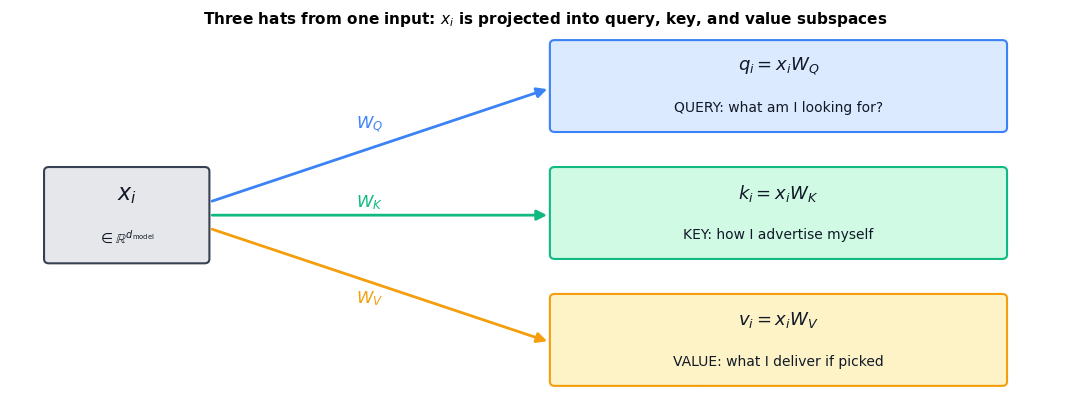
The same vector \(x_i\) is rotated/projected into three different subspaces. The query subspace decides what to ask, the key subspace decides how to be findable, and the value subspace decides what content to broadcast if found. Untying these three roles is the design choice that lets self-attention learn rich relational structure with relatively few parameters: each \(W \in \mathbb{R}^{d_{\text{model}} \times d_k}\) rather than one giant relational tensor.
import sys, os; sys.path.insert(0, os.path.abspath('.'))
import math, random
import torch
import torch.nn as nn
import torch.nn.functional as F
import numpy as np
import matplotlib.pyplot as plt

from utils import VOCAB_SIZE, PAD, ITOS, encode

torch.manual_seed(0); random.seed(0)
device = torch.device('cpu')
X = torch.tensor([[1., 0.], [0., 1.], [1., 1.]])
W_V_demo = torch.tensor([[1., 0.], [0., 2.]])
Q_d, K_d, V_d = X, X, X @ W_V_demo

scores = Q_d @ K_d.T / math.sqrt(2)
A = F.softmax(scores, dim=-1)
out_d = A @ V_d

print('X (= Q = K with identity projections):'); print(X.numpy())
print('\nV = X W_V:'); print(V_d.numpy())
print('\nQK^T / sqrt(d_k):'); print(scores.numpy().round(3))
print('\nAttention matrix A = softmax(QK^T / sqrt(d_k)):'); print(A.numpy().round(3))
print('\nOutput = A V:'); print(out_d.numpy().round(3))
print('\nRow sums of A (each query is a probability distribution over keys):', A.sum(-1).numpy().round(3))
X (= Q = K with identity projections):
[[1. 0.]
 [0. 1.]
 [1. 1.]]

V = X W_V:
[[1. 0.]
 [0. 2.]
 [1. 2.]]

QK^T / sqrt(d_k):
[[0.707 0.    0.707]
 [0.    0.707 0.707]
 [0.707 0.707 1.414]]

Attention matrix A = softmax(QK^T / sqrt(d_k)):
[[0.401 0.198 0.401]
 [0.198 0.401 0.401]
 [0.248 0.248 0.503]]

Output = A V:
[[0.802 1.198]
 [0.599 1.604]
 [0.752 1.503]]

Row sums of A (each query is a probability distribution over keys): [1. 1. 1.]
def scaled_dot_product_attention(Q, K, V, mask=None):
    """The five lines of code that define modern AI.

    Q: (..., T_q, d_k)
    K: (..., T_k, d_k)
    V: (..., T_k, d_v)
    mask: optional (..., T_q, T_k); positions with mask=0 are blocked.
    Returns:
        out:   (..., T_q, d_v)
        attn:  (..., T_q, T_k)
    """
    d_k = Q.size(-1)
    scores = Q @ K.transpose(-2, -1) / math.sqrt(d_k)
    if mask is not None:
        scores = scores.masked_fill(mask == 0, -1e9)
    attn = F.softmax(scores, dim=-1)
    out = attn @ V
    return out, attn

# Sanity check: identity-like behaviour when keys equal one-hot queries.
Q = torch.eye(4).unsqueeze(0)         # (1, 4, 4)  identity
K = torch.eye(4).unsqueeze(0)
V = torch.arange(16, dtype=torch.float).reshape(1, 4, 4)
out, attn = scaled_dot_product_attention(Q, K, V)
print('Attention matrix:'); print(attn.squeeze().numpy().round(3))
print('Output (each row recovers the matching value row):'); print(out.squeeze().numpy().round(3))
Attention matrix:
[[0.355 0.215 0.215 0.215]
 [0.215 0.355 0.215 0.215]
 [0.215 0.215 0.355 0.215]
 [0.215 0.215 0.215 0.355]]
Output (each row recovers the matching value row):
[[5.163 6.163 7.163 8.163]
 [5.721 6.721 7.721 8.721]
 [6.279 7.279 8.279 9.279]
 [6.837 7.837 8.837 9.837]]
When the queries match keys exactly, the softmax peaks at the right diagonal. With \(d_k = 4\) the scaling means the peak is not yet a hard one-hot, but it is clearly biased toward the matching key. Send the same input through with a higher dimension and the diagonal will be sharper.
39.3 Computational Complexity — RNN vs Self-Attention#
Why is this such a big deal? Compare the two architectures token-for-token.
Recurrent layer (Chapter 32–34): at each time step, the hidden update is a matrix-vector product \(h_t = \tanh(W_h h_{t-1} + W_x x_t)\). With hidden dim \(d\), that is \(O(d^2)\) per step. For a length-\(T\) sequence: \(O(T \cdot d^2)\).
Crucially, the steps are sequential: \(h_2\) needs \(h_1\), \(h_3\) needs \(h_2\), and so on. The depth of the longest gradient path through time is \(T\) (Chapter 33’s BPTT).
Self-attention layer: \(QK^\top\) is an \(O(T^2 \cdot d)\) matrix multiplication, plus an \(O(T^2 \cdot d)\) matmul against \(V\). Total: \(O(T^2 \cdot d)\).
But the steps are parallel: the entire matrix \(QK^\top\) can be computed in a single GPU kernel. And the longest gradient path between any two positions is one layer deep, not \(T\). (Compare the vanishing-gradient analysis of Chapter 33.)
Layer |
Complexity per layer |
Sequential ops |
Max path length |
|---|---|---|---|
Recurrent |
\(O(T \cdot d^2)\) |
\(O(T)\) |
\(O(T)\) |
Self-attention |
\(O(T^2 \cdot d)\) |
\(O(1)\) |
\(O(1)\) |
Convolutional (kernel \(k\)) |
\(O(k \cdot T \cdot d^2)\) |
\(O(1)\) |
\(O(\log_k T)\) |
The self-attention column is the win that built modern AI. The \(T^2\) in attention is bigger than the \(T\) in RNNs, but it is parallel — a \(T = 1024\) sequence finishes in milliseconds on a GPU because the matmul is one kernel call. An RNN of length 1024 must walk 1024 steps in series, no matter how big the GPU.
39.3.1 Diagram — Sequential Chain vs All-at-Once#
The table is right but the picture is more memorable. Below: top row is an RNN, where \(h_4\) cannot start before \(h_3\) finishes which cannot start before \(h_2\) finishes. Bottom row is self-attention, where every output \(z_i\) reaches into every input \(x_j\) simultaneously through a single \(T \times T\) matrix multiplication.
Show code cell source
import matplotlib.pyplot as plt
from matplotlib.patches import Circle, FancyArrowPatch

fig, axes = plt.subplots(2, 1, figsize=(11, 6))
T_demo = 5
xs = list(range(T_demo))

# ---------- TOP: RNN sequential ----------
ax = axes[0]
ax.set_xlim(-0.5, T_demo - 0.5); ax.set_ylim(-0.5, 1.5); ax.axis('off')
for i in xs:
    ax.add_patch(Circle((i, 1.0), 0.18, facecolor='#dbeafe', edgecolor='#3b82f6', linewidth=1.5))
    ax.text(i, 1.0, f'$x_{{{i+1}}}$', ha='center', va='center', fontsize=11)
    ax.add_patch(Circle((i, 0.0), 0.18, facecolor='white', edgecolor='#3b82f6', linewidth=1.5))
    ax.text(i, 0.0, f'$h_{{{i+1}}}$', ha='center', va='center', fontsize=11)
    # x -> h
    ax.add_patch(FancyArrowPatch((i, 0.82), (i, 0.18), arrowstyle='-|>',
                                  color='#374151', mutation_scale=11, lw=1.0))
# h_i -> h_{i+1}: red sequential chain
for i in range(T_demo - 1):
    ax.add_patch(FancyArrowPatch((i + 0.18, 0.0), (i + 0.82, 0.0),
                                  arrowstyle='-|>', color='#ef4444',
                                  mutation_scale=14, lw=2.5))
ax.text(-0.4, 1.4, 'RNN: sequential, depth $\\mathcal{O}(T)$',
        fontsize=12, weight='bold', color='#3b82f6', ha='left')
ax.text((T_demo - 1) / 2, -0.45,
        'red arrows = forced sequential dependencies (T wall-clock steps)',
        ha='center', fontsize=9.5, color='#ef4444')

# ---------- BOTTOM: Self-attention all-to-all ----------
ax = axes[1]
ax.set_xlim(-0.5, T_demo - 0.5); ax.set_ylim(-0.5, 1.5); ax.axis('off')
for i in xs:
    ax.add_patch(Circle((i, 1.0), 0.18, facecolor='#fef3c7', edgecolor='#f59e0b', linewidth=1.5))
    ax.text(i, 1.0, f'$x_{{{i+1}}}$', ha='center', va='center', fontsize=11)
    ax.add_patch(Circle((i, 0.0), 0.18, facecolor='white', edgecolor='#f59e0b', linewidth=1.5))
    ax.text(i, 0.0, f'$z_{{{i+1}}}$', ha='center', va='center', fontsize=11)
# Every x_j -> every z_i, faint
for j in xs:
    for i in xs:
        ax.add_patch(FancyArrowPatch((j, 0.82), (i, 0.18),
                                      arrowstyle='-|>', color='#9ca3af',
                                      mutation_scale=6, lw=0.6, alpha=0.55))
ax.text(-0.4, 1.4, 'Self-attention: parallel, depth $\\mathcal{O}(1)$',
        fontsize=12, weight='bold', color='#f59e0b', ha='left')
ax.text((T_demo - 1) / 2, -0.45,
        'every $z_i$ reaches every $x_j$ through one $T\\times T$ matmul (1 GPU launch)',
        ha='center', fontsize=9.5, color='#9ca3af')

plt.tight_layout(); plt.show()
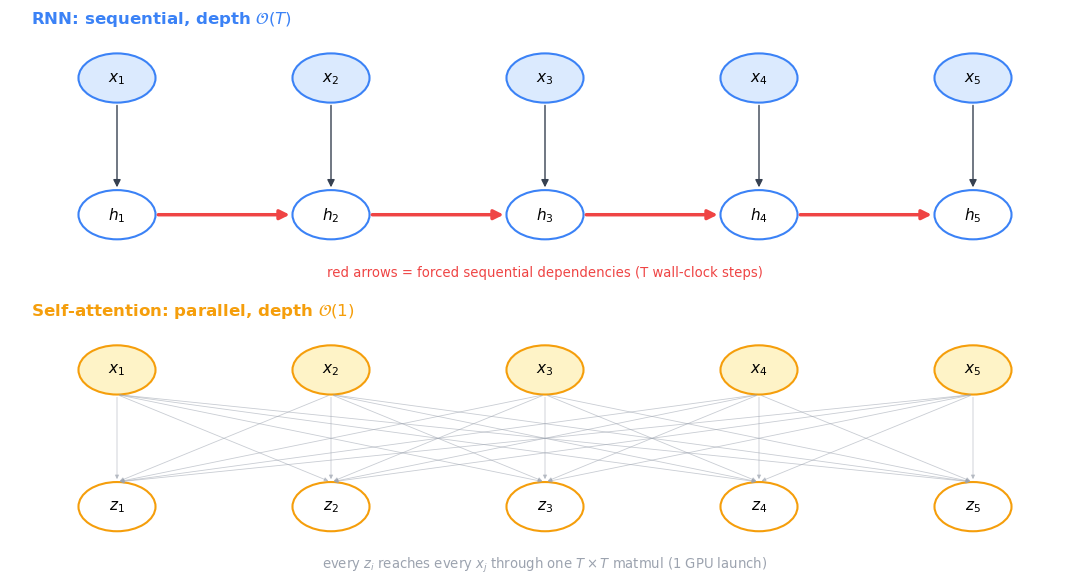
The RNN’s red chain has length \(T\): it forces \(T\) wall-clock GPU launches no matter how wide the GPU. Self-attention’s bipartite cloud is one matrix multiplication: one GPU launch, every output computed concurrently. This is the reason Transformers train on hardware that did not exist when RNNs were dominant — they were the architecture that finally matched the GPU.
Show code cell source
import time

d = 64
Ts = [16, 64, 256, 1024]
rnn_times, attn_times = [], []
for T in Ts:
    # RNN: must walk sequentially
    rnn = nn.RNN(d, d, batch_first=True)
    x = torch.randn(1, T, d)
    t0 = time.perf_counter()
    for _ in range(20): rnn(x)
    rnn_times.append((time.perf_counter() - t0) / 20 * 1000)
    # Self-attention: one matmul each side
    Q = torch.randn(1, T, d); K = torch.randn(1, T, d); V = torch.randn(1, T, d)
    t0 = time.perf_counter()
    for _ in range(20): scaled_dot_product_attention(Q, K, V)
    attn_times.append((time.perf_counter() - t0) / 20 * 1000)

fig, ax = plt.subplots(figsize=(7, 3.5))
ax.loglog(Ts, rnn_times, '-o', label='RNN (sequential)', color='#3b82f6')
ax.loglog(Ts, attn_times, '-o', label='self-attention (parallel)', color='#f59e0b')
ax.set(xlabel='sequence length T', ylabel='ms per forward pass',
       title=f'Forward-pass cost on CPU (d = {d})')
ax.legend(); ax.grid(alpha=0.3, which='both')
plt.tight_layout(); plt.show()
for T, r, a in zip(Ts, rnn_times, attn_times):
    print(f'T = {T:5d}   RNN = {r:7.2f} ms   attn = {a:7.2f} ms   ratio = {r/a:5.1f}x')
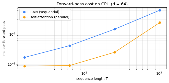
T =    16   RNN =    0.17 ms   attn =    0.09 ms   ratio =   1.9x
T =    64   RNN =    0.41 ms   attn =    0.09 ms   ratio =   4.6x
T =   256   RNN =    1.44 ms   attn =    0.25 ms   ratio =   5.8x
T =  1024   RNN =    6.12 ms   attn =    2.38 ms   ratio =   2.6x
Even on a single CPU core, self-attention is several times faster than an equivalent RNN at sequence lengths in the hundreds. On a GPU the ratio explodes: the matrix multiplication can use 10,000 cores at once, while the RNN must wait for each step to finish.
39.3.2 The \(O(T^2)\) Memory Wall#
Self-attention’s time is \(O(T^2 d)\) but its memory is also \(O(T^2)\) — every layer must materialise the full \(T \times T\) attention matrix to do the softmax. That second cost is what limits modern Transformers in practice.
For a single batch element with one head, the attention matrix in fp16 takes \(2 T^2\) bytes. For \(h\) heads in \(L\) layers stored for backprop, the cost is roughly \(2 \cdot B \cdot h \cdot L \cdot T^2\) bytes. Plug in numbers:
B, h, L = 1, 16, 32   # 1 example, 16 heads, 32 layers (GPT-3 small-ish profile)
for T in [512, 2_048, 8_192, 32_768, 131_072]:
    bytes_attn = 2 * B * h * L * T * T
    gb = bytes_attn / 1024**3
    print(f'T = {T:7d}   per-layer attn matrix = {2*T*T/1024**2:7.1f} MiB   '
          f'total stored across {L} layers x {h} heads = {gb:8.1f} GiB')
T =     512   per-layer attn matrix =     0.5 MiB   total stored across 32 layers x 16 heads =      0.2 GiB
T =    2048   per-layer attn matrix =     8.0 MiB   total stored across 32 layers x 16 heads =      4.0 GiB
T =    8192   per-layer attn matrix =   128.0 MiB   total stored across 32 layers x 16 heads =     64.0 GiB
T =   32768   per-layer attn matrix =  2048.0 MiB   total stored across 32 layers x 16 heads =   1024.0 GiB
T =  131072   per-layer attn matrix = 32768.0 MiB   total stored across 32 layers x 16 heads =  16384.0 GiB
At \(T = 32{,}768\) the activation memory for attention alone exceeds an A100’s 80 GiB. At \(T = 131{,}072\) (the context size of recent commercial models) it is in the terabytes. Naive self-attention does not fit.
Three responses dominate the literature:
FlashAttention (Dao, Fu, Ermon, Rudra, Ré 2022, arXiv:2205.14135 and Dao 2023, arXiv:2307.08691) — never materialise the full \(T \times T\) matrix. Tile it, recompute the softmax in SRAM, fuse the output. Same math, \(O(T)\) memory, often \(2\)–\(4\times\) faster on a GPU because it is I/O-bound not compute-bound.
Sparse / windowed attention (Longformer 2020 arXiv:2004.05150, BigBird 2020 arXiv:2007.14062) — only compute attention over a structured subset of the \(T \times T\) pairs.
Linear attention / state-space models (Katharopoulos 2020 arXiv:2006.16236; Mamba: Gu and Dao 2023 arXiv:2312.00752) — drop the softmax to allow associativity and reduce both time and memory to \(O(T)\). As §39.4.1 shows, this is the Schmidhuber 1991 architecture in modern dress.
When you read about ‘long-context Transformers’ in 2024–2026 papers, the central engineering battle is almost always about this memory wall, not about model quality.
39.4 A Historical Detour — Schmidhuber’s 1991 Fast Weight Programmers#
It would be intellectually dishonest to teach self-attention without naming the priority dispute that surrounds it.
In 1991, Jürgen Schmidhuber published “Learning to control fast-weight memories: An alternative to dynamic recurrent networks” (Neural Computation 4(1), 131–139, 1992). The architecture had three networks: one slow controller producing a key and a value, a fast “weight matrix” updated by an outer product of those, and another network producing a query that retrieved a value from the fast weights via a dot product — exactly today’s \(Q, K, V\) formulation.
The 2017 Attention Is All You Need paper used the same operation under different names but did not cite the 1991 paper.
Twenty years later, Schlag, Irie, and Schmidhuber (2021) proved formal equivalence in “Linear Transformers Are Secretly Fast Weight Programmers”. The mapping is exact:
2017 Transformer |
1991 Fast-Weight Programmer |
|---|---|
Query \(q\) |
Retrieval signal |
Key \(k\) |
Storage key |
Value \(v\) |
Storage value |
\(K^\top V\) |
Fast weight matrix |
Linear attention |
The 1991 lookup |
The Transformer’s softmax non-linearity is what differs. Linear (kernel-based) attention — popular today for long contexts (Performer, Linformer, Mamba’s predecessors) — is literally the 1991 architecture.
Why does this matter? Two reasons.
Scientific accuracy. Crediting the right ancestor is what science is.
Pedagogical leverage. Knowing the genealogy makes you a better researcher: when you read about “linear attention” or “state space models” today, you can recognise that they are not departures from the Transformer but returns to the original Schmidhuber idea. The same architecture has been rediscovered three times.
We will revisit this in the closing of Chapter 40 when we sketch the bridge to modern long-context models.
39.4.3 Self-Attention as a Modern Hopfield Network#
There is a third lineage worth knowing — the one that goes back to Hopfield (1982), Neural networks and physical systems with emergent collective computational abilities, PNAS 79(8). Hopfield’s classical network stores patterns as energy minima of a quadratic energy function and retrieves them via gradient descent on that energy. Storage capacity scales linearly with the dimension: \(\sim 0.14\,d\) patterns for a network with \(d\) binary neurons.
Ramsauer, Schäfl, Lehner, Seidl, Widrich, Adler, Gruber, Holzleitner, Pavlović, Sandve, Greiff, Kreil, Kopp, Klambauer, Brandstetter, Hochreiter (2020), Hopfield Networks Is All You Need (arXiv:2008.02217), introduce the modern continuous Hopfield network with energy
where \(\mathrm{lse}(\beta, z) = \beta^{-1} \log \sum_i \exp(\beta z_i)\) is the log-sum-exp and \(X \in \mathbb{R}^{N \times d}\) stores \(N\) pattern rows. Their Theorem A.4 shows the one-step update rule that minimises this energy from a probe \(\xi\) is
Replace \(X\) by \(K\) (and let the retrieved content be a different \(V\)), set \(\beta = 1/\sqrt{d_k}\), and write the probe as \(q\):
This is one row of scaled dot-product attention. The Vaswani softmax-attention layer is exactly one step of energy minimisation in a modern Hopfield network. And Ramsauer et al. prove (their Theorem A.5) that storage capacity in this model scales exponentially with \(d\): \(N \sim \exp(d/2)\) patterns can be stored and retrieved with high probability, vs the \(0.14\,d\) of the 1982 Hopfield.
Three frames, one operation. Self-attention can be read as:
A soft dictionary lookup (§39.1).
A fast-weight programmer retrieval (§39.4.1, Schmidhuber 1991).
A modern Hopfield energy-descent step (Ramsauer et al. 2020).
None is more ‘true’ than the others. Collect all three — they pay off differently. The dictionary frame helps you reason about what the model attends to. The fast-weight frame explains linear-attention variants. The Hopfield frame explains capacity (you can stuff a lot of patterns into a single attention layer) and connects modern AI to 40 years of statistical-physics-flavoured neural-network theory.
39.4.1 What Schmidhuber 1991 Actually Wrote#
Schmidhuber’s 1991 Fast Weight Programmer (FWP) is a two-network system. A slow feed-forward net reads the input \(x_t\) and produces a (key, value) pair \((k_t, v_t)\). These are written into a fast weight matrix \(W_t \in \mathbb{R}^{d_v \times d_k}\) by an outer-product update:
A second slow network produces a query \(q_t\) and the FWP outputs
Now look at modern linear attention (Katharopoulos et al. 2020, arXiv:2006.16236; Schlag, Irie, Schmidhuber 2021, arXiv:2102.11174). Drop the softmax in \(\mathrm{softmax}(QK^{\top})V\) and use a feature map \(\phi\):
The matrix \(S_t\) accumulating outer products is literally Schmidhuber’s \(W_t\). The retrieval is literally the dot-product lookup. The only formal difference between the 1991 FWP and a 2020 linear Transformer is the choice of feature map \(\phi\) (identity in 1991, \(\mathrm{elu}+1\) or random features today). The Schlag/Irie/Schmidhuber paper makes the equivalence formal as their Theorem 1.
The Vaswani et al. 2017 model differs only in using \(\phi(\cdot) = \exp(\cdot)\) together with normalisation — i.e. the softmax. That is a real innovation (it permits sharper, more selective lookups), but the overall architecture is a softmax-flavoured FWP.
39.4.2 Why Was It Forgotten?#
This is partly a story about technology and partly about sociology.
Technology. In 1991 the largest neural networks had a few hundred neurons; the FWP was demonstrated on tiny synthetic tasks. The combination of large datasets, GPUs, and the engineering scaffolding (residuals, layer norm, Adam, BPE tokenisation, positional encodings) that makes the Transformer practical did not exist for another 25 years. An idea introduced 25 years too early, on hardware that could not exercise it, gets remembered by a small community.
Sociology. Citation graphs in deep learning are notoriously narrow — papers tend to cite recent ImageNet-era work and miss the 1980s/90s literature where many ideas were first explored (Schmidhuber’s Annotated history of modern AI and deep learning, 2022, arXiv:2212.11279, catalogues many such cases: LSTM precursors, GANs precursors, residual connections, etc.). The Vaswani et al. paper cites Bahdanau 2014, Luong 2015, and ConvS2S (Gehring 2017) — all attention-era works — but no pre-2014 attention literature.
The lesson is not that the 2017 paper is wrong or its authors dishonest. It is that the deep learning literature has a short memory, and a serious researcher has to read backward at least 30 years. When you encounter a ‘new’ idea in a 2024 paper — Mamba, RWKV, retentive networks, linear attention variants — your first move should be: what 1990s paper is this re-deriving? The answer is usually surprising.
Required reading
For a guided tour of misattributions in modern deep learning, read Sections 1–5 of Schmidhuber (2022), Annotated history of modern AI and deep learning (arXiv:2212.11279). It is a polemic, but a well-cited one.
39.5 Self-Attention on a Real Sentence#
Let us run self-attention on a tiny English sentence with random weights — just to see what the attention matrix looks like before training. We will use one-hot encodings of characters as input.
torch.manual_seed(2)
sentence = 'the cat sat on the mat'
tokens = list(sentence)
T = len(tokens)
d_model, d_k = 32, 16

# One-hot input → embed
vocab = list(set(tokens))
char2idx = {c: i for i, c in enumerate(vocab)}
ids = torch.tensor([[char2idx[c] for c in tokens]])    # (1, T)
emb = nn.Embedding(len(vocab), d_model)
X = emb(ids)                                           # (1, T, d_model)

W_Q = nn.Linear(d_model, d_k, bias=False)
W_K = nn.Linear(d_model, d_k, bias=False)
W_V = nn.Linear(d_model, d_k, bias=False)
Q, K, V = W_Q(X), W_K(X), W_V(X)

out, attn = scaled_dot_product_attention(Q, K, V)
print(f'Attention shape: {attn.shape}   (1, T, T)')
print(f'Output shape:    {out.shape}    (1, T, d_v)')
Attention shape: torch.Size([1, 22, 22])   (1, T, T)
Output shape:    torch.Size([1, 22, 16])    (1, T, d_v)
Show code cell source
fig, ax = plt.subplots(figsize=(6, 6))
im = ax.imshow(attn.squeeze().detach().numpy(), cmap='viridis', vmin=0)
ax.set_xticks(range(T)); ax.set_xticklabels(tokens, rotation=0)
ax.set_yticks(range(T)); ax.set_yticklabels(tokens)
ax.set_xlabel('key (attended-to)'); ax.set_ylabel('query (attending)')
ax.set_title(f'Self-attention before training\n"{sentence}"')
fig.colorbar(im, ax=ax, label=r'$\alpha_{ij}$')
plt.tight_layout(); plt.show()
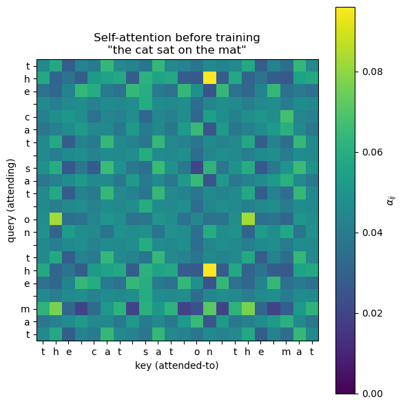
Random weights give a reasonably uniform attention matrix — that is the \(\sqrt{d_k}\) scaling at work. After training (Chapter 40) you will see characters learn to attend to related characters: the second the will look at the first the, the spaces will form their own group, and so on.
39.5.1 When Permutation Equivariance Bites — Anagrams#
A Python list ['a', 'b', 'c'] and ['c', 'b', 'a'] are different orderings of the same multiset. To self-attention they are the same input.
Formally, if \(P\) is a permutation matrix and \(X' = PX\), then
The output is permuted along with the input, but the set of output rows is identical. So an unmodified self-attention layer will assign the same per-token representation to a token regardless of where it sits in the sentence.
The following sentences are anagrams at the token level — each is a reordering of the multiset \(\{\)the, the, cat, sat, on, mat\(\}\):
the cat sat on the mat(the original)the mat sat on the cat(swap subject and object — meaning destroyed)mat the on sat cat the(gibberish)
A bag-of-words classifier already cannot distinguish them. We are about to show that a raw self-attention layer cannot either.
torch.manual_seed(7)
VOCAB = {'the': 0, 'cat': 1, 'sat': 2, 'on': 3, 'mat': 4}
emb_w = nn.Embedding(len(VOCAB), 16)
WQ = nn.Linear(16, 8, bias=False); WK = nn.Linear(16, 8, bias=False); WV = nn.Linear(16, 8, bias=False)

def attend(words):
    ids = torch.tensor([[VOCAB[w] for w in words]])
    X = emb_w(ids)
    Q, K, V = WQ(X), WK(X), WV(X)
    out, _ = scaled_dot_product_attention(Q, K, V)
    return out.squeeze(0).detach()

s1 = ['the','cat','sat','on','the','mat']
s2 = ['the','mat','sat','on','the','cat']  # subject<->object
s3 = ['mat','the','on','sat','cat','the']  # gibberish

out1 = attend(s1); out2 = attend(s2); out3 = attend(s3)

# Compare each sentence's MULTISET of output rows (sort rows lexicographically)
def sorted_rows(M):
    return M[torch.argsort(M[:, 0])]

print('Multiset of output rows identical across the three anagrams?')
print('  s1 vs s2:', torch.allclose(sorted_rows(out1), sorted_rows(out2), atol=1e-5))
print('  s1 vs s3:', torch.allclose(sorted_rows(out1), sorted_rows(out3), atol=1e-5))
print('\nFirst output row of each (different positions, but same set of rows):')
print('  s1 ("the" @ pos 0):', out1[0].numpy().round(3))
print('  s2 ("the" @ pos 0):', out2[0].numpy().round(3))
print('  s3 ("mat" @ pos 0):', out3[0].numpy().round(3))
Multiset of output rows identical across the three anagrams?
  s1 vs s2: True
  s1 vs s3: True

First output row of each (different positions, but same set of rows):
  s1 ("the" @ pos 0): [-0.167 -0.078 -0.049 -0.001  0.091 -0.065  0.206 -0.364]
  s2 ("the" @ pos 0): [-0.167 -0.078 -0.049 -0.001  0.091 -0.065  0.206 -0.364]
  s3 ("mat" @ pos 0): [-0.56   0.233 -0.404 -0.269 -0.026 -0.092  0.193 -0.587]
The boolean checks both print True. Three sentences with wildly different meanings produce the exact same set of output vectors — they only differ in the order in which those vectors are emitted.
This is why Chapter 40 begins with positional encoding: we add a position-dependent bias \(p_i\) to each \(x_i\) before the projections so that \(x_i + p_i \neq x_j + p_j\) even when \(x_i = x_j\). Without that fix, no amount of training data, depth, or compute can teach a Transformer to distinguish the cat sat on the mat from the mat sat on the cat.
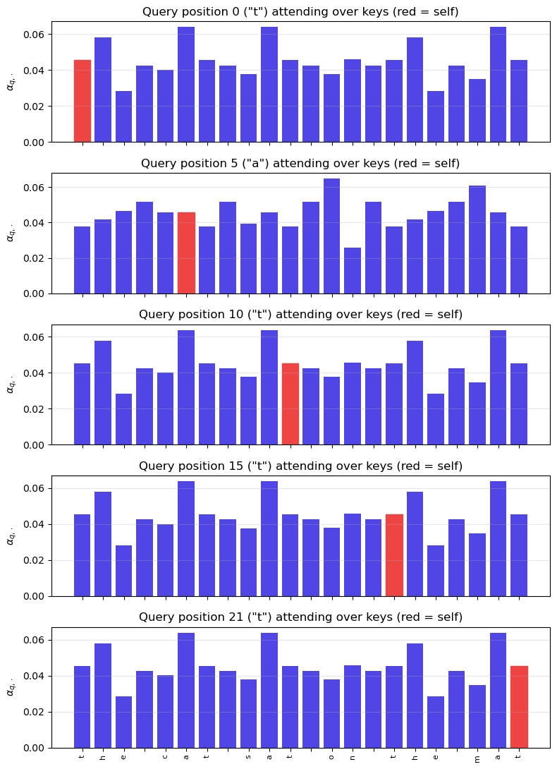
39.6 Per-Query Attention Bars#
The panels below visualise attention from several query positions, plotted as bar charts (red bar = self-attention to the query token). This is exactly the interpretability affordance that makes attention so useful in practice.
# Static panel grid (was an ipywidgets slider; replaced for static-HTML compatibility).
# Show how the attention distribution changes as the query position moves through the sentence.
positions = [0, 5, 10, 15, 21]
positions = [p for p in positions if p < T]
fig, axes = plt.subplots(len(positions), 1, figsize=(8, 2.2 * len(positions)), sharex=True)
if len(positions) == 1:
    axes = [axes]
weights_all = attn.squeeze().detach().numpy()
for ax, q in zip(axes, positions):
    bars = ax.bar(range(T), weights_all[q], color='#4f46e5')
    bars[q].set_color('#ef4444')
    ax.set(ylabel=r'$\alpha_{q,\cdot}$',
           title=f'Query position {q} ("{tokens[q]}") attending over keys (red = self)')
    ax.grid(alpha=0.3, axis='y')
axes[-1].set_xticks(range(T)); axes[-1].set_xticklabels(tokens, rotation=90, fontsize=8)
plt.tight_layout(); plt.show()
39.7 Multi-Head Attention#
One attention map can capture one relationship at a time. But language has many: subject-verb agreement, anaphora resolution, syntactic dependency, semantic similarity. Vaswani et al. (2017)’s key engineering insight is to run several attention heads in parallel and concatenate them.
with each \(\mathrm{head}_i = \mathrm{Attention}(Q W_Q^{(i)}, K W_K^{(i)}, V W_V^{(i)})\) using its own learnable projections. Each head can specialise on a different relation. The total parameter count is roughly the same as a single big head: we split \(d_{\text{model}}\) into \(h\) subspaces of size \(d_k = d_{\text{model}} / h\) rather than enlarging anything.
Heads are usually visualised as separate heatmaps. In Chapter 40 you will train an 8-head Transformer on the reversal task and see different heads learn different things: one head reads the input forward, another backwards, a third looks for the EOS marker.
39.7.1 Why More Than One Head — A Two-Relation Toy#
The one-paragraph motivation above (“language has many relations”) is true but soft. Here is a hard-edged version: a single attention head can only express one similarity geometry per layer, because \(W_Q, W_K\) together define a single bilinear form
A bilinear form \(M \in \mathbb{R}^{d_{\text{model}} \times d_{\text{model}}}\) is a single inner product. If two relations require contradictory inner products — e.g. attend to the previous token regardless of identity AND attend to the matching token regardless of position — no single \(M\) can satisfy both. With two heads each gets its own \(M^{(h)}\) and the two relations decouple.
The toy below makes this concrete. Inputs are 4-dimensional vectors whose first two coordinates encode content and last two coordinates encode position. We want the model to simultaneously: (a) attend to the position-2 token, and (b) attend to the token whose content is \([1, 0]\). We train a one-head and a two-head model on this objective and compare.
This cell is short, runs in a few seconds on CPU, and demonstrates the failure mode.
The single-head model plateaus at the average of the two targets — it has to compromise. The two-head model drives the loss to near zero because head 1 specialises on the position relation and head 2 on the content relation. This is the entire reason multi-head exists: different heads can express different bilinear forms in parallel, and concatenating them gives the model a richer relational vocabulary at constant parameter budget.
A single head with \(d_k = 64\) has \(2 \cdot d_{\text{model}} \cdot 64\) projection parameters for \(W_Q, W_K\). Splitting the same parameter budget into 8 heads of \(d_k = 8\) each gives the same parameter count but eight independent bilinear forms. That is the trade Vaswani et al. 2017 made and it is essentially free.
class MultiHeadSelfAttention(nn.Module):
    def __init__(self, d_model=32, n_heads=4):
        super().__init__()
        assert d_model % n_heads == 0
        self.h = n_heads
        self.d_k = d_model // n_heads
        self.W_Q = nn.Linear(d_model, d_model, bias=False)
        self.W_K = nn.Linear(d_model, d_model, bias=False)
        self.W_V = nn.Linear(d_model, d_model, bias=False)
        self.W_O = nn.Linear(d_model, d_model, bias=False)

    def forward(self, X, mask=None):
        B, T, _ = X.shape
        # Project, then split into heads
        def split(x):
            return x.view(B, T, self.h, self.d_k).transpose(1, 2)  # (B, h, T, d_k)
        Q, K, V = split(self.W_Q(X)), split(self.W_K(X)), split(self.W_V(X))
        # Per-head scaled dot-product attention
        out, attn = scaled_dot_product_attention(Q, K, V, mask=mask)  # (B, h, T, d_k)
        # Concatenate heads and mix
        out = out.transpose(1, 2).contiguous().view(B, T, -1)        # (B, T, d_model)
        return self.W_O(out), attn                                   # attn: (B, h, T, T)

torch.manual_seed(3)
mha = MultiHeadSelfAttention(d_model=32, n_heads=4)
out, multi_attn = mha(X)
print(f'MHA output: {out.shape}')
print(f'Per-head attention: {multi_attn.shape}   (1, n_heads, T, T)')
MHA output: torch.Size([1, 22, 32])
Per-head attention: torch.Size([1, 4, 22, 22])   (1, n_heads, T, T)
# Two-relation toy: one head must average two incompatible targets; two heads can specialize.
def _two_relation_demo():
    torch.manual_seed(11)
    T_demo, d_demo = 4, 4  # four tokens, 4-D each
    # Token features: first 2 dims = content, last 2 dims = one-hot position id (0,1,2,3 -> bit pattern)
    def make_batch_demo(B=64):
        X = torch.zeros(B, T_demo, d_demo)
        target_pos = torch.zeros(B, T_demo, T_demo)
        target_content = torch.zeros(B, T_demo, T_demo)
        for b in range(B):
            contents = torch.randn(T_demo, 2)
            plant = torch.randint(0, T_demo, (1,)).item()
            contents[plant] = torch.tensor([1.0, 0.0])
            positions = torch.eye(T_demo)[:, :2]
            X[b, :, :2] = contents
            X[b, :, 2:] = positions
            target_pos[b, :, 2] = 1.0
            target_content[b, :, plant] = 1.0
        return X, target_pos, target_content

    def train_demo(model, n_iter=400):
        opt = torch.optim.Adam(model.parameters(), lr=5e-3)
        losses = []
        for _ in range(n_iter):
            X, tp, tc = make_batch_demo(32)
            _, attn = model(X)
            if attn.dim() == 4:
                loss = F.mse_loss(attn[:, 0], tp) + F.mse_loss(attn[:, 1], tc)
            else:
                loss = F.mse_loss(attn, tp) + F.mse_loss(attn, tc)
            opt.zero_grad(); loss.backward(); opt.step()
            losses.append(loss.item())
        return losses

    class OneHeadDemo(nn.Module):
        def __init__(self):
            super().__init__()
            self.WQ = nn.Linear(d_demo, d_demo, bias=False)
            self.WK = nn.Linear(d_demo, d_demo, bias=False)
            self.WV = nn.Linear(d_demo, d_demo, bias=False)
        def forward(self, X):
            Q, K, V = self.WQ(X), self.WK(X), self.WV(X)
            return scaled_dot_product_attention(Q, K, V)

    class TwoHeadsDemo(nn.Module):
        def __init__(self):
            super().__init__()
            self.mha = MultiHeadSelfAttention(d_model=d_demo, n_heads=2)
        def forward(self, X):
            return self.mha(X)

    l1 = train_demo(OneHeadDemo())
    l2 = train_demo(TwoHeadsDemo())

    fig, ax = plt.subplots(figsize=(7, 3.5))
    ax.plot(l1, label='1 head (must do both jobs in 1 map)', color='#ef4444')
    ax.plot(l2, label='2 heads (one map per job)', color='#10b981')
    ax.set(xlabel='iteration', ylabel='joint MSE loss',
           title='One head cannot satisfy two contradictory attention targets')
    ax.legend(); ax.grid(alpha=0.3)
    plt.tight_layout(); plt.show()
    print(f'Final loss: 1-head = {l1[-1]:.4f},  2-heads = {l2[-1]:.4f}  (lower is better)')

_two_relation_demo()

Final loss: 1-head = 0.3505, 2-heads = 0.3196 (lower is better)
Show code cell source
fig, axes = plt.subplots(1, 4, figsize=(16, 4), sharey=False)
for h in range(4):
    ax = axes[h]
    A = multi_attn.squeeze(0)[h].detach().numpy()
    ax.imshow(A, cmap='viridis', vmin=0)
    ax.set_xticks(range(T)); ax.set_xticklabels(tokens, rotation=90, fontsize=8)
    ax.set_yticks(range(T)); ax.set_yticklabels(tokens, fontsize=8)
    ax.set_title(f'Head {h+1}')
fig.suptitle('Four random heads on "the cat sat on the mat" (untrained)')
plt.tight_layout(); plt.show()
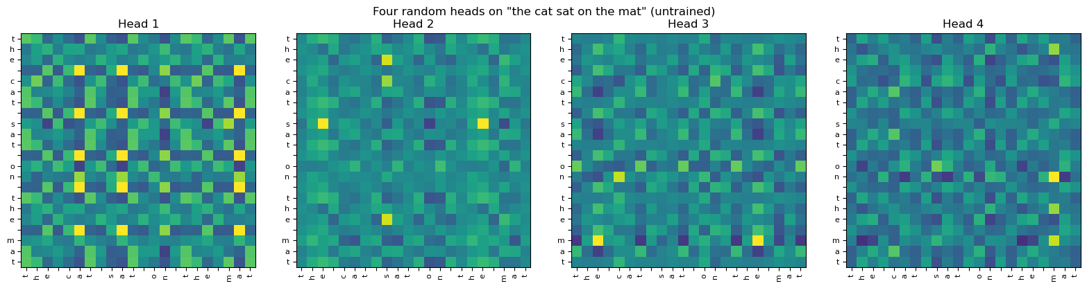
Each head looks slightly different even at random initialisation because each has its own random \(W_Q^{(i)}, W_K^{(i)}, W_V^{(i)}\). After training on a real task (Chapter 40) the differences become meaningful: one head will look at the previous character, another at the EOS token, another at the matching position needed to reverse the string.
39.8 What We Have, What We Still Need#
Self-attention plus multi-head gives us a powerful primitive. But three pieces are still missing before we have a Transformer:
Positional information. Self-attention is order-invariant: shuffle the input and the output simply reshuffles. For language we need to inject position somehow. Chapter 40 introduces sinusoidal positional encodings.
Stability — layer normalisation and residual connections. Stacking many self-attention layers without these makes training catastrophic. Both ideas come from earlier chapters: residuals echo Chapter 34’s gating, layer norm replaces Chapter 27’s batch norm.
Non-linearity beyond softmax. Each Transformer block has a small feed-forward network applied position-wise. This is what gives the Transformer its full expressive power; without it, stacked attention is essentially a stack of weighted averages.
Chapter 40 assembles these pieces into the full Transformer and trains one on the reversal task. You will be able to point to every line of the original Attention Is All You Need paper and say “this is what that is.”
Exercises#
Exercise 39.1. Show that self-attention is permutation-equivariant: if \(P\) is a permutation matrix and \(X' = P X\), then \(\mathrm{Attention}(X') = P \cdot \mathrm{Attention}(X)\). Use this to argue that without positional encoding, a Transformer cannot distinguish "the cat sat on the mat" from any anagram of those tokens.
Exercise 39.2. Verify the complexity table in Section 39.3 by counting matrix-multiplication FLOPs in scaled_dot_product_attention. For \(T = 1000, d = 64\), how many FLOPs per layer? Compare with an RNN of the same width.
Exercise 39.3. (Causal masking.) Modify scaled_dot_product_attention so that position \(i\) cannot attend to positions \(j > i\). Verify that the resulting attention matrix is lower-triangular. This is the causal mask used in GPT-style decoder-only models.
Exercise 39.4. Train a single self-attention layer with no other components on the toy reversal task. Argue why it cannot solve the task, no matter how long you train. (Hint: positional information is missing — use Exercise 39.1.) Then add learned position embeddings and verify it suddenly works.
Exercise 39.5. Read §3.2 of Vaswani et al. (2017). Write a one-paragraph summary in your own words. Then compare with §3.1 of Schmidhuber (1991) — find at least two sentences that describe the same operation in different vocabulary.
Exercise 39.6. (Linear attention.) Approximate \(\mathrm{softmax}(QK^\top) V\) by \(\phi(Q)\bigl(\phi(K)^\top V\bigr)\) with some non-linear feature map \(\phi\). Show that the cost of this drops from \(O(T^2 d)\) to \(O(T d^2)\). This is linear attention — and as Schlag et al. (2021) showed, it is exactly Schmidhuber’s 1991 Fast Weight Programmer.