Chapter 1: The McCulloch-Pitts Neuron (1943)

1. Introduction: The Meeting of Two Minds

In the early 1940s, an unlikely collaboration between a neurophysiologist and a self-taught teenage logician produced one of the most consequential papers in the history of computation and neuroscience.

Warren Sturgis McCulloch (1898–1969) was a Yale-trained physician and neurophysiologist who had spent years thinking about how the brain implements logical reasoning. He studied philosophy at Haverford College, medicine at Columbia, and had worked with Dusser de Barenne on the functional organization of the cerebral cortex. By the early 1940s, McCulloch was a professor of psychiatry at the University of Illinois at Chicago, obsessed with a question that had haunted him since his student days: “What is a number, that a man may know it, and a man, that he may know a number?”

Walter Harry Pitts (1923–1969) was a prodigy from Detroit who, at the age of 12, read Bertrand Russell and Alfred North Whitehead’s Principia Mathematica in the public library and wrote to Russell pointing out what he believed were errors. By 15, he had run away from home and was attending lectures by Rudolf Carnap at the University of Chicago — without ever formally enrolling. Carnap was so impressed that he employed Pitts as a research assistant. Pitts also came to the attention of the great mathematician-biologist Nicolas Rashevsky, who introduced him to McCulloch.

Their meeting, around 1941–1942, was electric. McCulloch had the biological insight and the philosophical ambition; Pitts had the mathematical formalism and the logical precision. Together, they produced:

McCulloch, W.S. and Pitts, W. (1943). “A Logical Calculus of the Ideas Immanent in Nervous Activity.” Bulletin of Mathematical Biophysics, 5(4), 115–133.

This paper proposed that neurons could be modeled as logical devices: each neuron either fires or does not (all-or-none), it receives inputs from other neurons, and it fires when the excitation exceeds a threshold — provided no inhibitory input is active. With this simple formalism, McCulloch and Pitts showed that suitably arranged networks could compute any Boolean function on binary inputs.

The intellectual milieu was extraordinary. Alan Turing had published his foundational paper on computable numbers in 1936. Kurt Godel’s incompleteness theorems (1931) had shaken the foundations of mathematics. Carnap, Russell, and the logical positivists were attempting to ground all knowledge in formal logic. McCulloch and Pitts synthesized these currents into a bridge between logic and neuroscience, showing that the brain — or at least an idealized version of it — could be understood as a computing machine.

The paper was initially ignored by most biologists (too mathematical) and most mathematicians (too biological). But it caught the eye of John von Neumann, who cited it in his design for the EDVAC computer, and Norbert Wiener, who made it a cornerstone of cybernetics. Through these channels, the McCulloch-Pitts neuron became the seed from which both artificial intelligence and computational neuroscience would grow.

Tip

The McCulloch-Pitts paper is a prime example of how breakthroughs often happen at the intersection of disciplines. McCulloch brought the biology; Pitts brought the logic. Neither could have written the paper alone. When studying neural networks, keep an eye on cross-disciplinary ideas — they remain the richest source of innovation.

2. The Five Axioms of the McCulloch-Pitts Neuron

McCulloch and Pitts based their model on five fundamental assumptions, each grounded in the neurophysiology known at the time:

Axiom 1: All-or-None Firing

\[x_i(t) \in \{0, 1\}\]

A neuron is a binary device. At any time step \(t\), neuron \(i\) is either firing (\(x_i(t) = 1\)) or silent (\(x_i(t) = 0\)). There are no intermediate states, no graded potentials, no continuous signals.

Biological motivation: The discovery of the action potential by Adrian (1926) and the subsequent work by Erlanger and Gasser showed that nerve impulses are stereotyped events — a neuron either generates a full action potential or none at all. This “all-or-none law” was well established by the 1940s.

Axiom 2: Fixed Threshold \(\theta\)

\[\theta_i \in \mathbb{Z}^{+} \quad \text{(a fixed positive integer for each neuron } i\text{)}\]

Each neuron \(i\) has a threshold \(\theta_i\). The neuron fires if and only if the total excitatory input meets or exceeds this threshold (subject to the inhibition constraint below). The threshold is a structural property of the neuron — it does not change over time.

Biological motivation: Real neurons have a threshold membrane potential (approximately \(-55\) mV for typical cortical neurons) that must be reached before an action potential is triggered. While real thresholds can adapt, McCulloch and Pitts treated them as fixed parameters.

Axiom 3: Synaptic Delay of One Time Step

\[\text{The output of neuron } j \text{ at time } t \text{ can influence neuron } i \text{ only at time } t+1.\]

There is a uniform, discrete time delay of exactly one step for signal transmission across every synapse. This discretization of time is what makes the model amenable to logical analysis.

Biological motivation: Synaptic transmission involves chemical or electrical processes that take a finite amount of time (typically 0.5–5 ms for chemical synapses). McCulloch and Pitts abstracted this into a single, uniform delay.

Axiom 4: Absolute Inhibition

\[\text{If any inhibitory input } x_k(t) = 1 \text{ for } k \in I_i, \text{ then } x_i(t+1) = 0, \text{ regardless of excitation.}\]

Inhibitory inputs have absolute veto power. Even a single active inhibitory synapse prevents the neuron from firing, no matter how many excitatory inputs are active. This is the most drastic simplification in the model.

Biological motivation: While real inhibition is not absolute, certain types of inhibition (shunting inhibition near the soma, or inhibition at the axon hillock) can effectively veto excitatory input. McCulloch and Pitts took the extreme case for mathematical tractability.

Axiom 5: Fixed Network Structure

\[\text{The connectivity and parameters of the network do not change over time.}\]

The network topology (which neurons connect to which), the synapse types (excitatory or inhibitory), and the thresholds are all fixed. There is no learning, no adaptation, no plasticity.

Biological motivation: This is the weakest axiom biologically. Even by the 1940s, it was suspected that synaptic connections could change. But McCulloch and Pitts were interested in what a fixed network could compute, not in how it might be constructed. Learning would come later (Hebb 1949, Rosenblatt 1958).

Danger

Biological Implausibility of the McCulloch-Pitts Model

While historically foundational, the M-P neuron is a drastic oversimplification of real biological neurons:

• Real neurons have graded potentials and continuous-valued membrane voltages, not binary states.

• Real synapses have variable strengths (weights) that change over time through plasticity mechanisms (LTP, LTD).

• Real inhibition is not absolute — it is graded and can be overcome by strong enough excitation.

• Real neurons have complex dendritic computations, not a simple sum-and-threshold.

• Real neural circuits have stochastic firing patterns and noise.

• There is no single clock synchronizing all neurons — real neural processing is asynchronous.

The M-P model should be understood as a logical idealization — useful for proving what is possible in principle, but not as a description of how real brains actually work.

3. Formal Definition

Let us now state the McCulloch-Pitts activation rule precisely.

Definition (McCulloch-Pitts Neuron)

A McCulloch-Pitts neuron \(i\) is characterized by:

• A set of excitatory input neurons \(E_i \subseteq \{1, 2, \ldots, n\}\)

• A set of inhibitory input neurons \(I_i \subseteq \{1, 2, \ldots, n\}\), with \(E_i \cap I_i = \emptyset\)

• A threshold \(\theta_i \in \mathbb{Z}^+\)

The activation rule is:

\[\begin{split}x_i(t+1) = \begin{cases} 1 & \text{if } \displaystyle\sum_{j \in E_i} x_j(t) \geq \theta_i \;\text{ and }\; \displaystyle\sum_{k \in I_i} x_k(t) = 0 \\[8pt] 0 & \text{otherwise} \end{cases}\end{split}\]

In words: neuron \(i\) fires at time \(t+1\) if and only if:

1. The number of active excitatory inputs at time \(t\) meets or exceeds the threshold \(\theta_i\), and

2. No inhibitory input is active at time \(t\).

Note on notation. Each excitatory input contributes a weight of exactly \(+1\). There are no variable weights — this is a crucial distinction from the later Perceptron model. The only parameters are the threshold \(\theta_i\) and the partition of inputs into excitatory and inhibitory sets.

Definition (McCulloch-Pitts Network)

A McCulloch-Pitts network is a directed graph \(G = (V, E)\) where:

• \(V = \{1, 2, \ldots, n\}\) is a set of M-P neurons

• \(E \subseteq V \times V\) is a set of directed edges, each labeled excitatory or inhibitory

• Each neuron \(i\) has a threshold \(\theta_i\)

The network is feedforward (acyclic) if the graph \(G\) contains no directed cycles; otherwise, it is recurrent (cyclic).

Tip

Notice that the M-P neuron has no variable weights — every excitatory connection contributes exactly \(+1\) to the sum, and every inhibitory connection is an absolute veto. This makes the model simpler to analyze mathematically, but it also means that a single M-P neuron can only compute threshold functions (also called linearly separable functions with unit weights). The introduction of variable weights by Rosenblatt (1958) was a major conceptual advance.

4. Python Implementation

We now implement the McCulloch-Pitts neuron in Python.

import numpy as np
import matplotlib.pyplot as plt
%matplotlib inline


class McCullochPittsNeuron:
    """
    A McCulloch-Pitts neuron.

    Parameters
    ----------
    threshold : int
        The firing threshold theta_i. The neuron fires when the number
        of active excitatory inputs >= threshold AND no inhibitory
        input is active.
    name : str, optional
        A human-readable name for the neuron (for display purposes).
    """

    def __init__(self, threshold, name=None):
        if threshold < 1:
            raise ValueError("Threshold must be a positive integer.")
        self.threshold = threshold
        self.name = name or f"MP(theta={threshold})"

    def activate(self, excitatory_inputs, inhibitory_inputs=None):
        """
        Compute the neuron output given inputs.

        Parameters
        ----------
        excitatory_inputs : list or array of {0, 1}
            The excitatory inputs at time t.
        inhibitory_inputs : list or array of {0, 1}, optional
            The inhibitory inputs at time t. If any is 1, output is 0.

        Returns
        -------
        int
            1 if the neuron fires, 0 otherwise.
        """
        if inhibitory_inputs is not None and any(inhibitory_inputs):
            return 0

        excitatory_sum = sum(excitatory_inputs)
        return 1 if excitatory_sum >= self.threshold else 0

    def __repr__(self):
        return f"McCullochPittsNeuron(threshold={self.threshold}, name='{self.name}')"


# Quick test
neuron = McCullochPittsNeuron(threshold=2, name="test")
print(f"Neuron: {neuron}")
print(f"activate([1, 1], [])  = {neuron.activate([1, 1], [])}")
print(f"activate([1, 0], [])  = {neuron.activate([1, 0], [])}")
print(f"activate([1, 1], [1]) = {neuron.activate([1, 1], [1])}")

Neuron: McCullochPittsNeuron(threshold=2, name='test')
activate([1, 1], [])  = 1
activate([1, 0], [])  = 0
activate([1, 1], [1]) = 0

5. Building Logic Gates

The power of the McCulloch-Pitts model becomes apparent when we realize that simple choices of thresholds and input types reproduce the fundamental logic gates.

AND Gate

To compute \(y = x_1 \wedge x_2\) (logical AND):

• Two excitatory inputs: \(x_1, x_2\)

• No inhibitory inputs

• Threshold \(\theta = 2\)

The neuron fires only when both inputs are 1 (since \(1 + 1 = 2 \geq 2\), but \(1 + 0 = 1 < 2\)).

\(x_1\)	\(x_2\)	\(x_1 \wedge x_2\)
0	0	0
0	1	0
1	0	0
1	1	1

OR Gate

To compute \(y = x_1 \vee x_2\) (logical OR):

• Two excitatory inputs: \(x_1, x_2\)

• No inhibitory inputs

• Threshold \(\theta = 1\)

The neuron fires when at least one input is 1.

\(x_1\)	\(x_2\)	\(x_1 \vee x_2\)
0	0	0
0	1	1
1	0	1
1	1	1

NOT Gate

To compute \(y = \neg x\) (logical NOT):

• One excitatory input that is always on (a bias input, always 1)

• One inhibitory input: \(x\)

• Threshold \(\theta = 1\)

When \(x = 0\): no inhibition, excitatory sum \(= 1 \geq 1\), so output \(= 1\). When \(x = 1\): inhibition is active, so output \(= 0\) regardless.

\(x\)	\(\neg x\)
0	1
1	0

Show code cell source Hide code cell source

# --- Building Logic Gates from McCulloch-Pitts Neurons ---
import numpy as np
import matplotlib.pyplot as plt
%matplotlib inline

# AND gate: threshold = 2, two excitatory inputs
and_gate = McCullochPittsNeuron(threshold=2, name="AND")

# OR gate: threshold = 1, two excitatory inputs
or_gate = McCullochPittsNeuron(threshold=1, name="OR")

# NOT gate: threshold = 1, one excitatory bias (always 1), one inhibitory input
not_gate = McCullochPittsNeuron(threshold=1, name="NOT")


def test_and_gate():
    print("=== AND Gate (theta=2) ===")
    print(f"{'x1':>4} {'x2':>4} {'AND':>5}")
    print("-" * 16)
    for x1 in [0, 1]:
        for x2 in [0, 1]:
            result = and_gate.activate([x1, x2])
            print(f"{x1:>4} {x2:>4} {result:>5}")
    print()


def test_or_gate():
    print("=== OR Gate (theta=1) ===")
    print(f"{'x1':>4} {'x2':>4} {'OR':>5}")
    print("-" * 16)
    for x1 in [0, 1]:
        for x2 in [0, 1]:
            result = or_gate.activate([x1, x2])
            print(f"{x1:>4} {x2:>4} {result:>5}")
    print()


def test_not_gate():
    print("=== NOT Gate (theta=1, bias=1, inhibitory) ===")
    print(f"{'x':>4} {'NOT':>5}")
    print("-" * 12)
    for x in [0, 1]:
        # Excitatory: always-on bias [1]
        # Inhibitory: the input x
        result = not_gate.activate([1], [x])
        print(f"{x:>4} {result:>5}")
    print()


test_and_gate()
test_or_gate()
test_not_gate()

=== AND Gate (theta=2) ===
  x1   x2   AND
----------------
   0    0     0
   0    1     0
   1    0     0
   1    1     1

=== OR Gate (theta=1) ===
  x1   x2    OR
----------------
   0    0     0
   0    1     1
   1    0     1
   1    1     1

=== NOT Gate (theta=1, bias=1, inhibitory) ===
   x   NOT
------------
   0     1
   1     0

Network Diagrams for AND, OR, and NOT Gates

The following visualization shows the network architecture of each basic gate, including nodes, edges, and weights.

Show code cell source Hide code cell source

import numpy as np
import matplotlib.pyplot as plt
import matplotlib.patches as mpatches
%matplotlib inline


def draw_mp_gate(ax, title, input_labels, input_types, threshold, output_label="y",
                 bias=False):
    """Draw a McCulloch-Pitts gate diagram."""
    ax.set_xlim(-0.5, 3.5)
    ax.set_ylim(-0.5, len(input_labels) + (1 if bias else 0) + 0.5)
    ax.set_aspect('equal')
    ax.axis('off')
    ax.set_title(title, fontsize=14, fontweight='bold', pad=10)

    all_labels = list(input_labels)
    all_types = list(input_types)
    if bias:
        all_labels.append("1 (bias)")
        all_types.append("exc")

    n = len(all_labels)
    neuron_x, neuron_y = 2.5, (n - 1) / 2.0

    # Draw neuron (output node)
    circle = plt.Circle((neuron_x, neuron_y), 0.35, fill=True,
                         facecolor='#E3F2FD', edgecolor='#1565C0', linewidth=2.5)
    ax.add_patch(circle)
    ax.text(neuron_x, neuron_y, f'$\\theta={threshold}$', ha='center', va='center',
            fontsize=11, fontweight='bold', color='#1565C0')

    # Draw output arrow
    ax.annotate(output_label, xy=(neuron_x + 0.35, neuron_y),
                xytext=(neuron_x + 1.0, neuron_y),
                fontsize=12, fontweight='bold', ha='left', va='center',
                arrowprops=dict(arrowstyle='->', color='black', lw=2))

    # Draw inputs and connections
    for i, (label, itype) in enumerate(zip(all_labels, all_types)):
        in_y = (n - 1) - i
        in_x = 0.0

        if 'bias' in label:
            color_fill, color_edge = '#FFF9C4', '#F9A825'
        elif itype == 'inh':
            color_fill, color_edge = '#FFCDD2', '#C62828'
        else:
            color_fill, color_edge = '#C8E6C9', '#2E7D32'

        circle_in = plt.Circle((in_x, in_y), 0.25, fill=True,
                                facecolor=color_fill, edgecolor=color_edge, linewidth=2)
        ax.add_patch(circle_in)
        ax.text(in_x, in_y, label, ha='center', va='center', fontsize=9, fontweight='bold')

        if itype == 'inh':
            ax.plot([in_x + 0.25, neuron_x - 0.35], [in_y, neuron_y],
                    'r--', linewidth=2, alpha=0.8)
            mid_label_x = (in_x + 0.25 + neuron_x - 0.35) / 2
            mid_label_y = (in_y + neuron_y) / 2 + 0.2
            ax.text(mid_label_x, mid_label_y, '-1 (veto)', fontsize=8, ha='center',
                    color='red', fontstyle='italic')
        else:
            ax.annotate('', xy=(neuron_x - 0.35, neuron_y),
                        xytext=(in_x + 0.25, in_y),
                        arrowprops=dict(arrowstyle='->', color='#2E7D32', lw=2, alpha=0.8))
            mid_label_x = (in_x + 0.25 + neuron_x - 0.35) / 2
            mid_label_y = (in_y + neuron_y) / 2 + 0.2
            ax.text(mid_label_x, mid_label_y, '+1', fontsize=9, ha='center',
                    color='#2E7D32', fontweight='bold')


fig, axes = plt.subplots(1, 3, figsize=(16, 5))

draw_mp_gate(axes[0], 'AND Gate', ['$x_1$', '$x_2$'], ['exc', 'exc'],
             threshold=2, output_label='$y$')
draw_mp_gate(axes[1], 'OR Gate', ['$x_1$', '$x_2$'], ['exc', 'exc'],
             threshold=1, output_label='$y$')
draw_mp_gate(axes[2], 'NOT Gate', ['$x$'], ['inh'],
             threshold=1, output_label='$y$', bias=True)

legend_elements = [
    mpatches.Patch(facecolor='#C8E6C9', edgecolor='#2E7D32', label='Excitatory input'),
    mpatches.Patch(facecolor='#FFCDD2', edgecolor='#C62828', label='Inhibitory input'),
    mpatches.Patch(facecolor='#FFF9C4', edgecolor='#F9A825', label='Bias (always 1)'),
    mpatches.Patch(facecolor='#E3F2FD', edgecolor='#1565C0', label='M-P Neuron'),
]
fig.legend(handles=legend_elements, loc='lower center', ncol=4, fontsize=10,
           framealpha=0.9, edgecolor='gray', bbox_to_anchor=(0.5, -0.02))

plt.tight_layout()
plt.subplots_adjust(bottom=0.12)
plt.show()

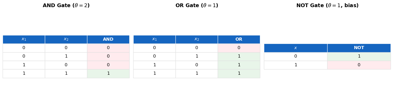
Truth Tables as Visual Summary

Below we display the truth tables for AND, OR, and NOT gates as styled matplotlib tables for easy reference.

Show code cell source Hide code cell source

import numpy as np
import matplotlib.pyplot as plt
%matplotlib inline


def draw_truth_table(ax, title, headers, rows, highlight_col=-1):
    """Draw a styled truth table using matplotlib."""
    ax.axis('off')
    ax.set_title(title, fontsize=14, fontweight='bold', pad=15)

    cell_text = [[str(v) for v in row] for row in rows]
    n_cols = len(headers)
    n_rows = len(rows)

    cell_colors = []
    for row in rows:
        row_colors = []
        for j, v in enumerate(row):
            if j == highlight_col:
                row_colors.append('#E8F5E9' if v == 1 else '#FFEBEE')
            else:
                row_colors.append('white')
        cell_colors.append(row_colors)

    table = ax.table(cellText=cell_text, colLabels=headers,
                     cellColours=cell_colors, loc='center',
                     cellLoc='center')
    table.auto_set_font_size(False)
    table.set_fontsize(12)
    table.scale(1.0, 1.8)

    for j in range(n_cols):
        cell = table[0, j]
        cell.set_facecolor('#1565C0')
        cell.set_text_props(color='white', fontweight='bold')
        cell.set_edgecolor('white')

    for i in range(1, n_rows + 1):
        for j in range(n_cols):
            cell = table[i, j]
            cell.set_edgecolor('#E0E0E0')


fig, axes = plt.subplots(1, 3, figsize=(15, 4))

draw_truth_table(axes[0], 'AND Gate ($\\theta=2$)',
                 ['$x_1$', '$x_2$', 'AND'],
                 [[0, 0, 0], [0, 1, 0], [1, 0, 0], [1, 1, 1]],
                 highlight_col=2)

draw_truth_table(axes[1], 'OR Gate ($\\theta=1$)',
                 ['$x_1$', '$x_2$', 'OR'],
                 [[0, 0, 0], [0, 1, 1], [1, 0, 1], [1, 1, 1]],
                 highlight_col=2)

draw_truth_table(axes[2], 'NOT Gate ($\\theta=1$, bias)',
                 ['$x$', 'NOT'],
                 [[0, 1], [1, 0]],
                 highlight_col=1)

plt.tight_layout()
plt.show()

6. Verification

Let us systematically verify each gate against its expected truth table.

Show code cell source Hide code cell source

def verify_gate(gate_name, gate_fn, truth_table):
    """Verify a gate function against an expected truth table."""
    all_pass = True
    for inputs, expected in truth_table.items():
        result = gate_fn(inputs)
        status = "PASS" if result == expected else "FAIL"
        if result != expected:
            all_pass = False
        print(f"  {gate_name}{inputs} = {result}  (expected {expected})  [{status}]")
    print(f"  >>> {'ALL TESTS PASSED' if all_pass else 'SOME TESTS FAILED'}")
    print()


def mp_and(inputs):
    x1, x2 = inputs
    return and_gate.activate([x1, x2])


def mp_or(inputs):
    x1, x2 = inputs
    return or_gate.activate([x1, x2])


def mp_not(inputs):
    (x,) = inputs
    return not_gate.activate([1], [x])


and_truth = {(0,0): 0, (0,1): 0, (1,0): 0, (1,1): 1}
or_truth  = {(0,0): 0, (0,1): 1, (1,0): 1, (1,1): 1}
not_truth = {(0,): 1, (1,): 0}

print("Verifying AND gate:")
verify_gate("AND", mp_and, and_truth)

print("Verifying OR gate:")
verify_gate("OR", mp_or, or_truth)

print("Verifying NOT gate:")
verify_gate("NOT", mp_not, not_truth)

Verifying AND gate:
  AND(0, 0) = 0  (expected 0)  [PASS]
  AND(0, 1) = 0  (expected 0)  [PASS]
  AND(1, 0) = 0  (expected 0)  [PASS]
  AND(1, 1) = 1  (expected 1)  [PASS]
  >>> ALL TESTS PASSED

Verifying OR gate:
  OR(0, 0) = 0  (expected 0)  [PASS]
  OR(0, 1) = 1  (expected 1)  [PASS]
  OR(1, 0) = 1  (expected 1)  [PASS]
  OR(1, 1) = 1  (expected 1)  [PASS]
  >>> ALL TESTS PASSED

Verifying NOT gate:
  NOT(0,) = 1  (expected 1)  [PASS]
  NOT(1,) = 0  (expected 0)  [PASS]
  >>> ALL TESTS PASSED

7. McCulloch-Pitts Network

To compose neurons into circuits, we need a network abstraction that handles the propagation of signals through layers of neurons.

class McCullochPittsNetwork:
    """
    A feedforward network of McCulloch-Pitts neurons organized in layers.

    Parameters
    ----------
    n_inputs : int
        Number of external inputs to the network.
    """

    def __init__(self, n_inputs):
        self.n_inputs = n_inputs
        self.layers = []

    def add_layer(self, layer_spec):
        """Add a layer of neurons to the network."""
        self.layers.append(layer_spec)

    def forward(self, inputs):
        """Propagate inputs through the network."""
        if len(inputs) != self.n_inputs:
            raise ValueError(
                f"Expected {self.n_inputs} inputs, got {len(inputs)}"
            )
        current_signals = list(inputs)
        for layer in self.layers:
            next_signals = []
            for spec in layer:
                neuron = spec['neuron']
                exc = [current_signals[i] for i in spec['excitatory']]
                inh = [current_signals[i] for i in spec['inhibitory']]
                output = neuron.activate(exc, inh)
                next_signals.append(output)
            current_signals = next_signals
        return current_signals

    def __repr__(self):
        desc = f"McCullochPittsNetwork(inputs={self.n_inputs}, layers={len(self.layers)})"
        for i, layer in enumerate(self.layers):
            neurons = [s['neuron'].name for s in layer]
            desc += f"\n  Layer {i}: {neurons}"
        return desc


# --- Example: Build an AND gate as a network ---
and_net = McCullochPittsNetwork(n_inputs=2)
and_net.add_layer([
    {
        'neuron': McCullochPittsNeuron(threshold=2, name='AND'),
        'excitatory': [0, 1],
        'inhibitory': []
    }
])

print(and_net)
print()
for x1 in [0, 1]:
    for x2 in [0, 1]:
        result = and_net.forward([x1, x2])
        print(f"AND({x1}, {x2}) = {result[0]}")

McCullochPittsNetwork(inputs=2, layers=1)
  Layer 0: ['AND']

AND(0, 0) = 0
AND(0, 1) = 0
AND(1, 0) = 0
AND(1, 1) = 1

8. Functional Completeness

Theorem (Functional Completeness)

The set of logic gates \(\{\text{AND}, \text{OR}, \text{NOT}\}\) is functionally complete: every Boolean function \(f: \{0,1\}^n \to \{0,1\}\) can be expressed as a composition of AND, OR, and NOT gates.

Proof

This is a classical result from propositional logic. The proof proceeds via the Disjunctive Normal Form (DNF) construction:

1. Given any Boolean function \(f: \{0,1\}^n \to \{0,1\}\), consider its truth table.

2. For each row where \(f = 1\), construct a minterm: a conjunction (AND) of all \(n\) variables, where variable \(x_i\) appears as itself if it is 1 in that row, or as \(\neg x_i\) if it is 0.

3. The function \(f\) is the disjunction (OR) of all such minterms.

For example, if \(f(0,1) = 1\) and \(f(1,0) = 1\) (and \(f = 0\) elsewhere), then:

\[f(x_1, x_2) = (\neg x_1 \wedge x_2) \vee (x_1 \wedge \neg x_2)\]

Since McCulloch-Pitts neurons can implement AND, OR, and NOT (as shown above), and any Boolean function can be decomposed into these gates, it follows that:

Corollary (M-P Universality for Boolean Functions)

For every Boolean function \(f: \{0,1\}^n \to \{0,1\}\), there exists a feedforward McCulloch-Pitts network that computes \(f\). \(\blacksquare\)

This is the essence of Theorem I from McCulloch and Pitts (1943) — though they stated it in the language of temporal propositional calculus rather than Boolean circuits.

9. Theorem I: Acyclic Universality

Theorem I (Acyclic Universality — McCulloch-Pitts, 1943)

For any temporal propositional expression (i.e., any Boolean function of inputs at a single preceding time step), there exists a feedforward McCulloch-Pitts network that computes it.

More precisely: Let \(f: \{0,1\}^n \to \{0,1\}\) be any Boolean function. Then there exists a feedforward M-P network with \(n\) inputs and one output such that for all \(\mathbf{x} \in \{0,1\}^n\), the output at time \(t+d\) (where \(d\) is the network depth) equals \(f(\mathbf{x})\) when \(\mathbf{x}\) is presented at time \(t\).

Proof (via DNF construction)

Let \(f: \{0,1\}^n \to \{0,1\}\) be arbitrary. We construct a feedforward M-P network in three layers:

Layer 0 (Input): The \(n\) input lines \(x_1, \ldots, x_n\).

Layer 1 (Negation): For each variable \(x_i\), create a NOT neuron computing \(\bar{x}_i\). This layer has \(n\) neurons (or fewer, if some variables do not need negation). After this layer, we have access to both \(x_i\) and \(\bar{x}_i\).

Layer 2 (Minterms): For each input \(\mathbf{a} = (a_1, \ldots, a_n) \in \{0,1\}^n\) with \(f(\mathbf{a}) = 1\), create an AND neuron. This neuron receives excitatory input from \(x_i\) if \(a_i = 1\), or from \(\bar{x}_i\) if \(a_i = 0\). Its threshold is \(n\) (all must be active). The number of such neurons equals \(|f^{-1}(1)|\), the number of ones in the truth table.

Layer 3 (Output): A single OR neuron that receives excitatory input from all minterm neurons in Layer 2. Its threshold is 1.

Correctness: For input \(\mathbf{x}\), exactly those minterm neurons in Layer 2 fire whose associated input pattern matches \(\mathbf{x}\), i.e., at most one neuron fires. The output OR neuron fires iff at least one minterm neuron fires, which happens iff \(f(\mathbf{x}) = 1\). \(\blacksquare\)

Complexity. The DNF construction uses at most \(n + 2^n + 1\) neurons. This is worst-case optimal for some functions (e.g., parity), but many functions admit much smaller networks.

Tip

The DNF construction gives us a universal but potentially expensive recipe. The key insight is that universality exists — we can build any Boolean function — but efficiency is a separate question. This tension between expressiveness and efficiency runs through all of neural network theory, from McCulloch-Pitts to modern deep learning.

10. DNF Construction Example: Majority-of-3

The majority function on 3 inputs outputs 1 if and only if at least 2 of the 3 inputs are 1:

\[\begin{split}\text{MAJ}(x_1, x_2, x_3) = \begin{cases} 1 & \text{if } x_1 + x_2 + x_3 \geq 2 \\ 0 & \text{otherwise} \end{cases}\end{split}\]

Its truth table has ones at: \((0,1,1), (1,0,1), (1,1,0), (1,1,1)\).

The DNF is:

\[\text{MAJ} = (\bar{x}_1 \wedge x_2 \wedge x_3) \vee (x_1 \wedge \bar{x}_2 \wedge x_3) \vee (x_1 \wedge x_2 \wedge \bar{x}_3) \vee (x_1 \wedge x_2 \wedge x_3)\]

However, note that we can implement majority much more efficiently with a single M-P neuron: threshold \(\theta = 2\), three excitatory inputs. This works because the M-P neuron already computes a threshold function!

Let us implement both the DNF construction and the direct construction, and verify they agree.

Show code cell source Hide code cell source

# --- DNF Construction for Majority-of-3 ---

def build_majority_dnf():
    """Build majority-of-3 using the DNF construction."""
    net_with_bias = McCullochPittsNetwork(n_inputs=4)  # x1, x2, x3, bias

    # Layer 1: NOT gates (3) + pass-throughs (3)
    layer1 = [
        {'neuron': McCullochPittsNeuron(1, 'NOT_x1'), 'excitatory': [3], 'inhibitory': [0]},
        {'neuron': McCullochPittsNeuron(1, 'NOT_x2'), 'excitatory': [3], 'inhibitory': [1]},
        {'neuron': McCullochPittsNeuron(1, 'NOT_x3'), 'excitatory': [3], 'inhibitory': [2]},
        {'neuron': McCullochPittsNeuron(1, 'PASS_x1'), 'excitatory': [0], 'inhibitory': []},
        {'neuron': McCullochPittsNeuron(1, 'PASS_x2'), 'excitatory': [1], 'inhibitory': []},
        {'neuron': McCullochPittsNeuron(1, 'PASS_x3'), 'excitatory': [2], 'inhibitory': []},
    ]
    net_with_bias.add_layer(layer1)

    # Layer 2: Minterm AND gates
    layer2 = [
        {'neuron': McCullochPittsNeuron(3, 'M_011'), 'excitatory': [0, 4, 5], 'inhibitory': []},
        {'neuron': McCullochPittsNeuron(3, 'M_101'), 'excitatory': [3, 1, 5], 'inhibitory': []},
        {'neuron': McCullochPittsNeuron(3, 'M_110'), 'excitatory': [3, 4, 2], 'inhibitory': []},
        {'neuron': McCullochPittsNeuron(3, 'M_111'), 'excitatory': [3, 4, 5], 'inhibitory': []},
    ]
    net_with_bias.add_layer(layer2)

    # Layer 3: OR gate
    layer3 = [
        {'neuron': McCullochPittsNeuron(1, 'OR_out'), 'excitatory': [0, 1, 2, 3], 'inhibitory': []}
    ]
    net_with_bias.add_layer(layer3)
    return net_with_bias


def build_majority_direct():
    """Majority-of-3 as a single M-P neuron with threshold 2."""
    net = McCullochPittsNetwork(n_inputs=3)
    net.add_layer([
        {'neuron': McCullochPittsNeuron(2, 'MAJ'), 'excitatory': [0, 1, 2], 'inhibitory': []}
    ])
    return net


maj_dnf = build_majority_dnf()
maj_direct = build_majority_direct()

print("DNF construction:")
print(maj_dnf)
print()
print("Direct construction:")
print(maj_direct)
print()

print(f"{'x1':>4} {'x2':>4} {'x3':>4} {'DNF':>5} {'Direct':>7} {'Match':>6}")
print("-" * 34)
all_match = True
for x1 in [0, 1]:
    for x2 in [0, 1]:
        for x3 in [0, 1]:
            dnf_result = maj_dnf.forward([x1, x2, x3, 1])[0]
            direct_result = maj_direct.forward([x1, x2, x3])[0]
            match = dnf_result == direct_result
            if not match:
                all_match = False
            print(f"{x1:>4} {x2:>4} {x3:>4} {dnf_result:>5} {direct_result:>7} {'OK' if match else 'FAIL':>6}")

print(f"\nAll outputs match: {all_match}")

DNF construction:
McCullochPittsNetwork(inputs=4, layers=3)
  Layer 0: ['NOT_x1', 'NOT_x2', 'NOT_x3', 'PASS_x1', 'PASS_x2', 'PASS_x3']
  Layer 1: ['M_011', 'M_101', 'M_110', 'M_111']
  Layer 2: ['OR_out']

Direct construction:
McCullochPittsNetwork(inputs=3, layers=1)
  Layer 0: ['MAJ']

  x1   x2   x3   DNF  Direct  Match
----------------------------------
   0    0    0     0       0     OK
   0    0    1     0       0     OK
   0    1    0     0       0     OK
   0    1    1     1       1     OK
   1    0    0     0       0     OK
   1    0    1     1       1     OK
   1    1    0     1       1     OK
   1    1    1     1       1     OK

All outputs match: True

11. Exercises

Exercise 1.1: NAND and NOR Gates

Implement NAND (\(\overline{x_1 \wedge x_2}\)) and NOR (\(\overline{x_1 \vee x_2}\)) gates using McCulloch-Pitts neurons.

Verify your implementations against the expected truth tables:

\(x_1\)	\(x_2\)	NAND	NOR
0	0	1	1
0	1	1	0
1	0	1	0
1	1	0	0

Hint

Each of these can be implemented with a single M-P neuron. For NAND, think about what combination of threshold, excitatory inputs, and inhibitory inputs gives you the right truth table. One approach: use a bias input (always 1) as the excitatory input (\(\theta = 1\)), and make both \(x_1\) and \(x_2\) inhibitory. Then the neuron fires whenever neither input is active, plus… but wait, inhibition is absolute (any single inhibitory input vetoes). So the neuron fires iff both \(x_1 = 0\) and \(x_2 = 0\). That is NOR, not NAND!

For NAND, you may need a two-neuron construction: first compute AND, then negate with NOT.

For NOR: the output should be 1 only when both inputs are 0. This can be done with a single neuron: make both inputs inhibitory, add a bias, and set \(\theta = 1\).

Exercise 1.2: Half-Adder

Build a half-adder circuit using M-P neurons. A half-adder takes two 1-bit inputs \(x_1, x_2\) and produces:

• Sum \(S = x_1 \oplus x_2\) (XOR)

• Carry \(C = x_1 \wedge x_2\) (AND)

\(x_1\)	\(x_2\)	Sum	Carry
0	0	0	0
0	1	1	0
1	0	1	0
1	1	0	1

Hint

The carry is just AND (\(\theta = 2\), both excitatory). The sum is XOR, which requires a multi-neuron network. Recall the decomposition: \(\text{XOR}(x_1, x_2) = (x_1 \wedge \neg x_2) \vee (\neg x_1 \wedge x_2)\). You will need NOT gates (which require a bias input), AND gates, and an OR gate.

Exercise 1.3: Minimum Neurons for XOR

What is the minimum number of McCulloch-Pitts neurons needed to compute XOR?

Claim: No single M-P neuron can compute XOR.

Proof: Consider XOR\((x_1, x_2)\). We need output 0 for \((0,0)\) and \((1,1)\), but output 1 for \((0,1)\) and \((1,0)\).

If neither input is inhibitory, then the excitatory sum is \(x_1 + x_2\). For \((0,1)\) and \((1,0)\), the sum is 1; for \((1,1)\), the sum is 2. We need \(\theta \leq 1\) (to fire on sum 1) but also need the neuron not to fire on sum 2 — impossible, since \(2 \geq \theta\) whenever \(1 \geq \theta\).

If one input, say \(x_2\), is inhibitory, then XOR\((1, 0)\) should give 1 (which works: \(x_1 = 1 \geq \theta\) with no inhibition) and XOR\((0, 1)\) should give 1 (but \(x_2\) is now inhibitory and active, so output must be 0). Contradiction.

The minimum network for XOR uses 5 neurons in the straightforward DNF construction (2 NOT, 2 AND, 1 OR), though it can also be done with fewer using clever constructions.

Hint

Can you do it with fewer than 5 neurons? Consider a construction using inhibitory inputs more cleverly. One approach: use 2 neurons in the first layer (one that fires for \(x_1 \wedge \neg x_2\) using inhibition, and one for \(\neg x_1 \wedge x_2\) using inhibition), plus 1 OR neuron. That gives 3 neurons — but the first two neurons each need a bias input.

12. Summary and Key Takeaways

In this chapter, we have studied the McCulloch-Pitts neuron (1943), the first formal model of neural computation:

1. The model is remarkably simple. A neuron is a binary threshold unit with excitatory and inhibitory inputs. It fires when the excitatory count reaches the threshold and no inhibitory input is active.

2. Single neurons compute threshold functions. AND, OR, and NOT (with a bias) are all threshold functions and can each be realized by a single M-P neuron.

3. Networks are universal. Since \(\{\text{AND}, \text{OR}, \text{NOT}\}\) is functionally complete, any Boolean function can be computed by a feedforward M-P network. This is Theorem I of the original paper.

4. The DNF construction provides a systematic (but potentially exponential) method for building a network for any Boolean function.

5. XOR cannot be computed by a single neuron. This limitation of single threshold units foreshadows the deeper results of Minsky and Papert (1969).

6. There is no learning. The network structure, thresholds, and connections are all fixed. How to find the right network for a given task remains an open question at this stage — one that will drive the next several decades of research.

Tip

The McCulloch-Pitts neuron teaches us a fundamental lesson about modeling: start with the simplest possible abstraction that captures the essential phenomenon. McCulloch and Pitts stripped away everything — continuous potentials, variable weights, learning, noise — and were left with a model simple enough to prove theorems about, yet powerful enough to compute any Boolean function. This strategy of radical simplification followed by gradual enrichment is a recurring pattern in science.

What comes next:

• In Chapter 2, we will explore the construction of complex circuits, recurrent networks, and the question of Turing equivalence.

• In later parts of this course, we will see how Hebb (1949) introduced a learning rule, how Rosenblatt (1958) built the Perceptron with adjustable weights, and how the backpropagation algorithm (1986) finally solved the training problem for multi-layer networks.

13. References

1. McCulloch, W.S. and Pitts, W. (1943). “A Logical Calculus of the Ideas Immanent in Nervous Activity.” Bulletin of Mathematical Biophysics, 5(4), 115–133. The foundational paper. Dense but rewarding. Focus on Theorems I–III and the examples of logic gate construction.

2. Kleene, S.C. (1956). “Representation of Events in Nerve Nets and Finite Automata.” In C.E. Shannon and J. McCarthy (eds.), Automata Studies, Princeton University Press, 3–41. Kleene reformulated and extended the McCulloch-Pitts results using the theory of regular events and finite automata. This paper introduced regular expressions.

3. Piccinini, G. (2004). “The First Computational Theory of Mind and Brain: A Close Look at McCulloch and Pitts’s ‘Logical Calculus of Ideas Immanent in Nervous Activity’.” Synthese, 141(2), 175–215. An excellent philosophical and historical analysis of the McCulloch-Pitts paper, placing it in the context of the logical positivist movement and the emergence of computationalism.

4. Arbib, M.A. (1987). Brains, Machines, and Mathematics, 2nd ed. Springer-Verlag. Chapter 2 provides a clear modern exposition of McCulloch-Pitts neurons and their properties.

5. Abraham, T.H. (2002). “(Physio)logical circuits: The intellectual origins of the McCulloch-Pitts neural networks.” Journal of the History of the Behavioral Sciences, 38(1), 3–25. Detailed intellectual history of how McCulloch and Pitts came to their collaboration.