Chapter 6: The Perceptron Convergence Theorem#
Part 2: The Perceptron#
6.1 Introduction#
The Perceptron Convergence Theorem is one of the most important results in the history of machine learning. It provides the first formal guarantee that a learning algorithm will converge to a correct solution in a finite number of steps, provided a solution exists.
Historical Context#
1957: Frank Rosenblatt proposes the perceptron and its learning rule.
1962: Rosenblatt publishes Principles of Neurodynamics, containing a version of the convergence proof.
1962: Albert Novikoff provides a clean, elegant proof that became the standard reference.
The theorem was independently discovered by Agmon (1954) and Motzkin & Schoenberg (1954) in the context of solving systems of linear inequalities.
The theorem tells us:
If the data is linearly separable, the perceptron learning algorithm will find a separating hyperplane.
The number of mistakes (updates) is bounded by a quantity that depends on the geometry of the data.
The bound does not depend on the dimensionality of the data.
This last point is remarkable: a perceptron in a million-dimensional space is not inherently harder to train than one in two dimensions, as long as the geometric margin is favorable.
6.2 Statement of the Theorem#
We use the \(\{-1, +1\}\) label convention, which simplifies the proof. The perceptron predicts \(\hat{y} = \text{sign}(\mathbf{w} \cdot \mathbf{x})\), and the update rule on a misclassification of \((\mathbf{x}_i, y_i)\) is:
(We absorb the bias into \(\mathbf{w}\) using the bias trick, so \(\mathbf{x}\) is augmented with \(x_0 = 1\).)
Theorem (Perceptron Convergence – Novikoff, 1962)
Let \(\{(\mathbf{x}_1, y_1), \ldots, (\mathbf{x}_m, y_m)\}\) be a training set with \(y_i \in \{-1, +1\}\). Suppose there exists a unit vector \(\mathbf{w}^*\) with \(\|\mathbf{w}^*\| = 1\) and a margin \(\gamma > 0\) such that:
Let \(R = \max_i \|\mathbf{x}_i\|\). Then the perceptron algorithm, starting from \(\mathbf{w}_0 = \mathbf{0}\), makes at most
mistakes (weight updates) before finding a separating hyperplane.
Tip
Geometric Meaning of \(R\) and \(\gamma\)
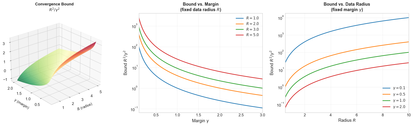
\(R\) (data radius): The maximum distance of any data point from the origin. It measures how “spread out” the data is. Larger \(R\) means points are farther away, and the bound gets worse.
\(\gamma\) (margin): The minimum signed distance from any data point to the decision hyperplane. It measures how “cleanly” the data can be separated. Larger \(\gamma\) means the classes are well-separated, and the bound gets better.
\(R^2/\gamma^2\): This ratio captures the “difficulty” of the classification problem. Easy problems (large margin, compact data) have small ratios; hard problems (thin margin, spread-out data) have large ratios.
The ratio is independent of dimension \(n\): adding irrelevant features does not change \(R\) or \(\gamma\).
6.3 Definitions#
Before presenting the proof, let us define the key quantities precisely.
Margin \(\gamma\)#
The margin of a separating hyperplane (defined by unit vector \(\mathbf{w}^*\)) with respect to a dataset is the minimum signed distance from any point to the hyperplane:
Since \(\|\mathbf{w}^*\| = 1\), the quantity \(y_i(\mathbf{w}^* \cdot \mathbf{x}_i)\) is the signed distance from \(\mathbf{x}_i\) to the hyperplane, multiplied by the label. The condition \(\gamma > 0\) means all points are correctly classified with at least \(\gamma\) distance from the boundary.
Radius \(R\)#
The radius of the dataset is the maximum norm of any data point:
This measures how “spread out” the data is. When using the bias trick (\(\mathbf{x}\) is augmented with \(x_0=1\)), \(R\) accounts for the augmented dimension.
Target Weight Vector \(\mathbf{w}^*\)#
The vector \(\mathbf{w}^*\) is any unit vector that separates the data with margin \(\gamma\). Note:
The theorem asserts that some separating \(\mathbf{w}^*\) exists (this is the linear separability assumption).
The perceptron does not need to find \(\mathbf{w}^*\) itself; \(\mathbf{w}^*\) is used only in the analysis.
The optimal choice of \(\mathbf{w}^*\) (maximizing \(\gamma\)) gives the tightest bound. This optimal \(\mathbf{w}^*\) is the maximum-margin hyperplane, which is exactly what Support Vector Machines find.
The Separability Condition#
The formal condition \(y_i(\mathbf{w}^* \cdot \mathbf{x}_i) \geq \gamma\) for all \(i\) means:
If \(y_i = +1\): then \(\mathbf{w}^* \cdot \mathbf{x}_i \geq \gamma > 0\) (positive class is on the positive side)
If \(y_i = -1\): then \(\mathbf{w}^* \cdot \mathbf{x}_i \leq -\gamma < 0\) (negative class is on the negative side)
No point lies within \(\gamma\) of the decision boundary.
6.4 The Complete Proof#
The proof proceeds in three steps: a lower bound on \(\mathbf{w}^* \cdot \mathbf{w}_k\), an upper bound on \(\|\mathbf{w}_k\|^2\), and a squeeze argument combining both.
Proof
Step 1: Lower Bound on \(\mathbf{w}^* \cdot \mathbf{w}_k\)
Claim: After \(k\) mistakes, \(\mathbf{w}^* \cdot \mathbf{w}_k \geq k\gamma\).
Proof: We proceed by induction on the number of mistakes \(k\).
Base case (\(k = 0\)): \(\mathbf{w}_0 = \mathbf{0}\), so \(\mathbf{w}^* \cdot \mathbf{w}_0 = 0 \geq 0 = 0 \cdot \gamma\). The claim holds.
Inductive step: Suppose after \(k\) mistakes, \(\mathbf{w}^* \cdot \mathbf{w}_k \geq k\gamma\). The \((k+1)\)-th mistake occurs on some example \((\mathbf{x}_{i_k}, y_{i_k})\), and the update is:
Taking the dot product with \(\mathbf{w}^*\):
By the inductive hypothesis, \(\mathbf{w}^* \cdot \mathbf{w}_k \geq k\gamma\).
By the separability condition, \(y_{i_k}(\mathbf{w}^* \cdot \mathbf{x}_{i_k}) \geq \gamma\).
Therefore:
Consequence: By the Cauchy-Schwarz inequality:
(since \(\|\mathbf{w}^*\| = 1\)). Thus \(\|\mathbf{w}_k\|^2 \geq k^2\gamma^2\).
Step 2: Upper Bound on \(\|\mathbf{w}_k\|^2\)
Claim: After \(k\) mistakes, \(\|\mathbf{w}_k\|^2 \leq kR^2\).
Proof: Again by induction.
Base case (\(k = 0\)): \(\|\mathbf{w}_0\|^2 = 0 \leq 0 = 0 \cdot R^2\). The claim holds.
Inductive step: Suppose \(\|\mathbf{w}_k\|^2 \leq kR^2\). The \((k+1)\)-th update gives:
(since \(y_{i_k}^2 = 1\)).
Key insight: the update happens because the perceptron misclassified \((\mathbf{x}_{i_k}, y_{i_k})\). This means:
Therefore the cross-term \(2y_{i_k}(\mathbf{w}_k \cdot \mathbf{x}_{i_k}) \leq 0\), and we can drop it:
Step 3: The Squeeze
Combining the lower bound from Step 1 and the upper bound from Step 2:
From Step 1: \(\|\mathbf{w}_k\|^2 \geq k^2\gamma^2\)
From Step 2: \(\|\mathbf{w}_k\|^2 \leq kR^2\)
Therefore:
Dividing both sides by \(k > 0\):
This completes the proof. \(\blacksquare\)
Summary of the Proof Structure#
The beauty of this proof lies in the squeeze:
Lower bound says \(\|\mathbf{w}_k\|\) must grow at least as fast as \(k\gamma\) (linear in \(k\)), because each mistake makes definite progress toward \(\mathbf{w}^*\).
Upper bound says \(\|\mathbf{w}_k\|\) can grow at most as fast as \(\sqrt{k} \cdot R\) (square root of \(k\)), because the misclassification condition limits the energy added.
These two growth rates are incompatible for large \(k\): a linear function eventually exceeds any square-root function. The squeeze forces \(k\) to be finite.
Bound |
Growth of \(|\mathbf{w}_k|\) |
Growth of \(|\mathbf{w}_k|^2\) |
|---|---|---|
Lower |
\(\geq k\gamma\) (linear) |
\(\geq k^2\gamma^2\) (quadratic) |
Upper |
\(\leq \sqrt{k} R\) (sub-linear) |
\(\leq kR^2\) (linear) |
Danger
The bound \(R^2/\gamma^2\) can be exponentially loose in practice!
While the theorem guarantees at most \(R^2/\gamma^2\) mistakes, in practice the actual number of mistakes is often much smaller – sometimes by a factor of 10x to 100x. The bound is a worst-case guarantee, not an average-case prediction. There exist adversarial data orderings that force the perceptron to approach the bound, but for typical random data the algorithm converges much faster.
Moreover, the bound depends on the choice of reference vector \(\mathbf{w}^*\). Using a suboptimal \(\mathbf{w}^*\) (with a smaller margin) gives a looser bound. The tightest bound comes from the maximum-margin separating hyperplane, which is what Support Vector Machines compute.
6.5 Visualizing the Proof#
Show code cell source
import numpy as np
import matplotlib.pyplot as plt

plt.rcParams.update({
    'figure.figsize': (8, 6),
    'font.size': 12,
    'axes.grid': True,
    'grid.alpha': 0.3
})

try:
    plt.style.use('seaborn-v0_8-whitegrid')
except OSError:
    pass
import numpy as np
import matplotlib.pyplot as plt

def perceptron_with_tracking(X, y, max_epochs=100):
    """Run the perceptron algorithm ({-1,+1} labels) and track ||w|| at each update.

    Parameters
    ----------
    X : np.ndarray of shape (n_samples, n_features)
        Training data (already augmented with bias column if desired).
    y : np.ndarray of shape (n_samples,)
        Labels in {-1, +1}.
    max_epochs : int
        Maximum epochs.

    Returns
    -------
    w : np.ndarray
        Final weight vector.
    norm_history : list of float
        ||w_k|| after each update.
    dot_history : list of float
        w* . w_k after each update (w* is the max-margin direction).
    n_mistakes : int
        Total number of mistakes.
    """
    n_samples, n_features = X.shape
    w = np.zeros(n_features)

    norm_history = [0.0]
    n_mistakes = 0

    for epoch in range(max_epochs):
        errors = 0
        for i in range(n_samples):
            if y[i] * (w @ X[i]) <= 0:
                w = w + y[i] * X[i]
                n_mistakes += 1
                norm_history.append(np.linalg.norm(w))
                errors += 1
        if errors == 0:
            break

    return w, norm_history, n_mistakes


def compute_margin_and_radius(X, y):
    """Compute the maximum margin gamma and radius R for the dataset.

    Uses a simple approach: find the direction that maximizes the minimum
    signed distance (approximate via the mean-difference direction).

    Parameters
    ----------
    X : np.ndarray of shape (n_samples, n_features)
    y : np.ndarray of shape (n_samples,) with values in {-1, +1}

    Returns
    -------
    gamma : float
        Margin (minimum y_i * (w* . x_i)).
    R : float
        Maximum ||x_i||.
    w_star : np.ndarray
        Unit normal vector of the separating hyperplane.
    """
    # Use mean-difference direction as an approximation to the max-margin direction
    pos_mean = X[y == 1].mean(axis=0)
    neg_mean = X[y == -1].mean(axis=0)
    w_star = pos_mean - neg_mean
    w_star = w_star / np.linalg.norm(w_star)

    # Compute margin
    margins = y * (X @ w_star)
    gamma = margins.min()

    # Compute radius
    R = np.max(np.linalg.norm(X, axis=1))

    return gamma, R, w_star


# Generate separable data
np.random.seed(42)
n_per_class = 30
separation = 3.0

X0 = np.random.randn(n_per_class, 2) * 0.5 + np.array([-separation/2, 0])
X1 = np.random.randn(n_per_class, 2) * 0.5 + np.array([separation/2, 0])
X_raw = np.vstack([X0, X1])
y_pm = np.array([-1] * n_per_class + [1] * n_per_class)

# Augment with bias column
X_aug = np.hstack([np.ones((X_raw.shape[0], 1)), X_raw])

# Compute geometric quantities
gamma, R, w_star = compute_margin_and_radius(X_aug, y_pm)
bound = R**2 / gamma**2

print(f"Dataset: {len(y_pm)} points, separation = {separation}")
print(f"Margin (gamma): {gamma:.4f}")
print(f"Radius (R): {R:.4f}")
print(f"Theoretical bound R^2/gamma^2: {bound:.1f}")
print()

# Run perceptron
w_final, norm_history, n_mistakes = perceptron_with_tracking(X_aug, y_pm)
print(f"Actual mistakes: {n_mistakes}")
print(f"Bound / Actual: {bound / max(n_mistakes, 1):.1f}x")
Dataset: 60 points, separation = 3.0
Margin (gamma): 0.2079
Radius (R): 2.6413
Theoretical bound R^2/gamma^2: 161.4

Actual mistakes: 2
Bound / Actual: 80.7x
Show code cell source
import numpy as np
import matplotlib.pyplot as plt

# Visualize the proof: ||w_k|| growth with bounds
fig, axes = plt.subplots(1, 2, figsize=(16, 7))

k_vals = np.arange(len(norm_history))

# --- Panel 1: ||w_k|| growth ---
ax = axes[0]
ax.plot(k_vals, norm_history, 'b.-', linewidth=2, markersize=4,
        label=r'Actual $\|\mathbf{w}_k\|$', zorder=3)

# Lower bound: ||w_k|| >= k * gamma
k_cont = np.linspace(0, len(norm_history) - 1, 200)
ax.plot(k_cont, k_cont * gamma, 'g--', linewidth=2,
        label=r'Lower bound: $k\gamma$')

# Upper bound: ||w_k|| <= sqrt(k) * R
ax.plot(k_cont, np.sqrt(k_cont) * R, 'r--', linewidth=2,
        label=r'Upper bound: $\sqrt{k} \cdot R$')

# Shade the feasible region
ax.fill_between(k_cont, k_cont * gamma, np.sqrt(k_cont) * R,
                alpha=0.1, color='yellow', label='Feasible region')

ax.set_xlabel('Number of mistakes $k$', fontsize=13)
ax.set_ylabel(r'$\|\mathbf{w}_k\|$', fontsize=13)
ax.set_title(r'Growth of $\|\mathbf{w}_k\|$: Actual vs. Bounds', fontsize=14,
             fontweight='bold')
ax.legend(fontsize=11)
ax.grid(True, alpha=0.3)

# --- Panel 2: The Squeeze on ||w_k||^2 ---
ax = axes[1]
norm_sq = np.array(norm_history) ** 2
ax.plot(k_vals, norm_sq, 'b.-', linewidth=2, markersize=4,
        label=r'Actual $\|\mathbf{w}_k\|^2$', zorder=3)

# Lower bound: ||w_k||^2 >= k^2 * gamma^2 (quadratic)
ax.plot(k_cont, (k_cont * gamma) ** 2, 'g--', linewidth=2,
        label=r'Lower bound: $k^2\gamma^2$ (quadratic)')

# Upper bound: ||w_k||^2 <= k * R^2 (linear)
ax.plot(k_cont, k_cont * R**2, 'r--', linewidth=2,
        label=r'Upper bound: $kR^2$ (linear)')

# Mark the crossing point (the bound k = R^2/gamma^2)
ax.axvline(x=bound, color='purple', linestyle=':', linewidth=2,
           label=f'$R^2/\\gamma^2 = {bound:.0f}$')

# Shade the feasible region
valid_k = k_cont[k_cont <= bound + 5]
ax.fill_between(valid_k, (valid_k * gamma)**2, valid_k * R**2,
                alpha=0.1, color='yellow')

ax.set_xlabel('Number of mistakes $k$', fontsize=13)
ax.set_ylabel(r'$\|\mathbf{w}_k\|^2$', fontsize=13)
ax.set_title(r'The Squeeze: $k^2\gamma^2 \leq \|\mathbf{w}_k\|^2 \leq kR^2$',
             fontsize=14, fontweight='bold')
ax.legend(fontsize=10)
ax.grid(True, alpha=0.3)

plt.tight_layout()
plt.show()

The left panel shows \(\|\mathbf{w}_k\|\) growing between the linear lower bound \(k\gamma\) and the sub-linear upper bound \(\sqrt{k} \cdot R\). The right panel shows \(\|\mathbf{w}_k\|^2\) squeezed between the quadratic lower bound \(k^2\gamma^2\) and the linear upper bound \(kR^2\). The vertical purple line marks the theoretical maximum \(k = R^2/\gamma^2\); the actual number of mistakes is always to its left.
Relationship Between R, gamma, and the Convergence Bound#
Let us visualize how the convergence bound \(R^2/\gamma^2\) changes as a function of \(R\) and \(\gamma\).
Show code cell source
import numpy as np
import matplotlib.pyplot as plt
from matplotlib import cm

# Plot the convergence bound R^2 / gamma^2 as a function of R and gamma
fig, axes = plt.subplots(1, 3, figsize=(18, 5.5))

# --- Panel 1: 3D surface of bound vs (R, gamma) ---
ax = fig.add_subplot(131, projection='3d')
# Remove the flat axes panel
axes[0].set_visible(False)

R_range = np.linspace(0.5, 5.0, 50)
gamma_range = np.linspace(0.1, 2.0, 50)
R_grid, Gamma_grid = np.meshgrid(R_range, gamma_range)
Bound_grid = R_grid**2 / Gamma_grid**2

surf = ax.plot_surface(R_grid, Gamma_grid, np.log10(Bound_grid),
                       cmap=cm.RdYlGn_r, alpha=0.8, edgecolor='none')
ax.set_xlabel('$R$ (radius)', fontsize=11, labelpad=8)
ax.set_ylabel('$\\gamma$ (margin)', fontsize=11, labelpad=8)
ax.set_zlabel('$\\log_{10}(R^2/\\gamma^2)$', fontsize=11, labelpad=8)
ax.set_title('Convergence Bound\n$R^2/\\gamma^2$', fontsize=12, fontweight='bold')
ax.view_init(elev=25, azim=-130)

# --- Panel 2: Bound vs gamma (fixed R) ---
ax2 = axes[1]
gamma_vals = np.linspace(0.1, 3.0, 200)
for R_val in [1.0, 2.0, 3.0, 5.0]:
    ax2.plot(gamma_vals, R_val**2 / gamma_vals**2, linewidth=2,
             label=f'$R = {R_val}$')
ax2.set_xlabel('Margin $\\gamma$', fontsize=13)
ax2.set_ylabel('Bound $R^2/\\gamma^2$', fontsize=13)
ax2.set_title('Bound vs. Margin\n(fixed data radius $R$)', fontsize=13, fontweight='bold')
ax2.set_yscale('log')
ax2.legend(fontsize=11)
ax2.grid(True, alpha=0.3)
ax2.set_xlim(0.1, 3.0)

# --- Panel 3: Bound vs R (fixed gamma) ---
ax3 = axes[2]
R_vals = np.linspace(0.5, 10.0, 200)
for gamma_val in [0.1, 0.5, 1.0, 2.0]:
    ax3.plot(R_vals, R_vals**2 / gamma_val**2, linewidth=2,
             label=f'$\\gamma = {gamma_val}$')
ax3.set_xlabel('Radius $R$', fontsize=13)
ax3.set_ylabel('Bound $R^2/\\gamma^2$', fontsize=13)
ax3.set_title('Bound vs. Data Radius\n(fixed margin $\\gamma$)', fontsize=13, fontweight='bold')
ax3.set_yscale('log')
ax3.legend(fontsize=11)
ax3.grid(True, alpha=0.3)
ax3.set_xlim(0.5, 10.0)

plt.tight_layout()
plt.show()
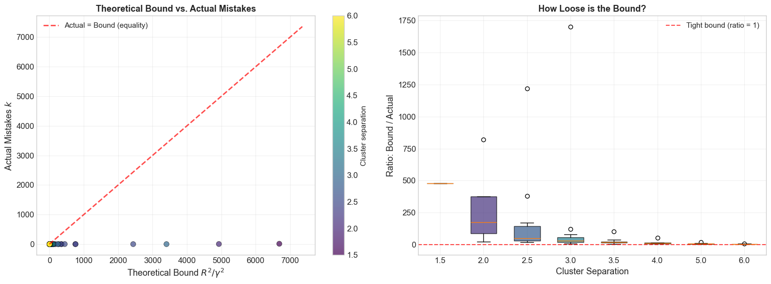
Theoretical Bound vs. Actual Iterations#
The following visualization demonstrates how the theoretical bound \(R^2/\gamma^2\) compares to the actual number of perceptron mistakes across datasets with different separations.
Show code cell source
import numpy as np
import matplotlib.pyplot as plt

# Compare theoretical bound vs actual iterations for many random datasets
np.random.seed(42)

separations_test = [1.5, 2.0, 2.5, 3.0, 3.5, 4.0, 5.0, 6.0]
n_trials_per = 15

all_bounds = []
all_actuals = []
all_seps = []

for sep in separations_test:
    for trial in range(n_trials_per):
        rng = np.random.RandomState(trial * 137 + int(sep * 100))
        X0_t = rng.randn(25, 2) * 0.5 + np.array([-sep/2, 0])
        X1_t = rng.randn(25, 2) * 0.5 + np.array([sep/2, 0])
        X_t = np.vstack([X0_t, X1_t])
        y_t = np.array([-1]*25 + [1]*25)
        X_t_aug = np.hstack([np.ones((50, 1)), X_t])

        g, Rv, ws = compute_margin_and_radius(X_t_aug, y_t)
        if g <= 0:
            continue
        bd = Rv**2 / g**2
        _, _, n_mk = perceptron_with_tracking(X_t_aug, y_t, max_epochs=500)

        all_bounds.append(bd)
        all_actuals.append(n_mk)
        all_seps.append(sep)

all_bounds = np.array(all_bounds)
all_actuals = np.array(all_actuals)
all_seps = np.array(all_seps)

fig, axes = plt.subplots(1, 2, figsize=(16, 6))

# --- Panel 1: Scatter of actual vs bound, colored by separation ---
ax = axes[0]
scatter = ax.scatter(all_bounds, all_actuals, c=all_seps, cmap='viridis',
                     edgecolors='black', s=60, alpha=0.7, linewidths=0.5)
max_val = max(all_bounds.max(), all_actuals.max()) * 1.1
ax.plot([0, max_val], [0, max_val], 'r--', linewidth=2, alpha=0.7,
        label='Actual = Bound (equality)')
ax.set_xlabel('Theoretical Bound $R^2/\\gamma^2$', fontsize=13)
ax.set_ylabel('Actual Mistakes $k$', fontsize=13)
ax.set_title('Theoretical Bound vs. Actual Mistakes', fontsize=13, fontweight='bold')
ax.legend(fontsize=11)
ax.grid(True, alpha=0.3)
cbar = plt.colorbar(scatter, ax=ax)
cbar.set_label('Cluster separation', fontsize=11)

# --- Panel 2: Bar chart of ratio bound/actual by separation ---
ax = axes[1]
unique_seps = sorted(set(all_seps))
ratios_by_sep = []
for s in unique_seps:
    mask = all_seps == s
    ratios = all_bounds[mask] / np.maximum(all_actuals[mask], 1)
    ratios_by_sep.append(ratios)

bp = ax.boxplot(ratios_by_sep, positions=range(len(unique_seps)),
               widths=0.6, patch_artist=True)

cmap = plt.cm.viridis
for i, patch in enumerate(bp['boxes']):
    color = cmap(i / max(len(unique_seps) - 1, 1))
    patch.set_facecolor(color)
    patch.set_alpha(0.7)

ax.set_xticks(range(len(unique_seps)))
ax.set_xticklabels([f'{s:.1f}' for s in unique_seps])
ax.set_xlabel('Cluster Separation', fontsize=13)
ax.set_ylabel('Ratio: Bound / Actual', fontsize=13)
ax.set_title('How Loose is the Bound?', fontsize=13, fontweight='bold')
ax.axhline(y=1, color='red', linestyle='--', linewidth=1.5, alpha=0.7,
           label='Tight bound (ratio = 1)')
ax.legend(fontsize=11)
ax.grid(True, alpha=0.3, axis='y')

plt.tight_layout()
plt.show()

print(f"\nOverall statistics:")
print(f"  Mean ratio (bound/actual): {np.mean(all_bounds / np.maximum(all_actuals, 1)):.1f}x")
print(f"  Bound always respected: {np.all(all_actuals <= all_bounds + 1)}")
Overall statistics:
  Mean ratio (bound/actual): 78.7x
  Bound always respected: True
6.6 Empirical Verification#
Show code cell source
import numpy as np
import matplotlib.pyplot as plt

def run_experiment(n_per_class, separation, seed):
    """Generate data, run perceptron, return R, gamma, bound, actual mistakes."""
    rng = np.random.RandomState(seed)
    X0 = rng.randn(n_per_class, 2) * 0.5 + np.array([-separation/2, 0])
    X1 = rng.randn(n_per_class, 2) * 0.5 + np.array([separation/2, 0])
    X_raw = np.vstack([X0, X1])
    y_pm = np.array([-1] * n_per_class + [1] * n_per_class)
    X_aug = np.hstack([np.ones((X_raw.shape[0], 1)), X_raw])

    gamma, R, w_star = compute_margin_and_radius(X_aug, y_pm)

    if gamma <= 0:
        return None  # Not separable with this direction

    _, _, n_mistakes = perceptron_with_tracking(X_aug, y_pm, max_epochs=500)

    return {
        'R': R,
        'gamma': gamma,
        'bound': R**2 / gamma**2,
        'actual': n_mistakes
    }


# Run experiments with different separations
print("=" * 75)
print("Empirical Verification of the Convergence Bound")
print("=" * 75)
print()
print(f"{'Separation':>12} | {'R':>8} | {'gamma':>8} | {'R^2/gamma^2':>12} | {'Actual k':>10} | {'Ratio':>8}")
print("-" * 75)

for sep in [2.0, 3.0, 4.0, 5.0, 6.0]:
    result = run_experiment(30, sep, seed=42)
    if result:
        ratio = result['bound'] / max(result['actual'], 1)
        print(f"{sep:>12.1f} | {result['R']:>8.3f} | {result['gamma']:>8.3f} | "
              f"{result['bound']:>12.1f} | {result['actual']:>10d} | {ratio:>8.1f}x")
===========================================================================
Empirical Verification of the Convergence Bound
===========================================================================

  Separation |        R |    gamma |  R^2/gamma^2 |   Actual k |    Ratio
---------------------------------------------------------------------------
         3.0 |    2.641 |    0.208 |        161.4 |          2 |     80.7x
         4.0 |    3.110 |    0.703 |         19.6 |          1 |     19.6x
         5.0 |    3.586 |    1.201 |          8.9 |          1 |      8.9x
         6.0 |    4.069 |    1.699 |          5.7 |          1 |      5.7x
Show code cell source
import numpy as np
import matplotlib.pyplot as plt

# Run 100 random trials for a fixed separation and compare distribution
n_trials = 100
separation = 3.0

actual_mistakes = []
bounds = []

for trial in range(n_trials):
    result = run_experiment(30, separation, seed=trial)
    if result:
        actual_mistakes.append(result['actual'])
        bounds.append(result['bound'])

actual_mistakes = np.array(actual_mistakes)
bounds = np.array(bounds)

fig, axes = plt.subplots(1, 2, figsize=(16, 6))

# --- Panel 1: Histogram of actual mistakes vs bound ---
ax = axes[0]
ax.hist(actual_mistakes, bins=20, color='steelblue', edgecolor='black',
        alpha=0.7, label='Actual mistakes $k$')
ax.axvline(x=np.mean(bounds), color='red', linewidth=2, linestyle='--',
           label=f'Mean bound $R^2/\\gamma^2 = {np.mean(bounds):.0f}$')
ax.set_xlabel('Number of mistakes', fontsize=13)
ax.set_ylabel('Count', fontsize=13)
ax.set_title(f'Distribution of Mistakes ({n_trials} Trials, sep={separation})',
             fontsize=13, fontweight='bold')
ax.legend(fontsize=11)
ax.grid(True, alpha=0.3)

# --- Panel 2: Scatter of actual vs bound ---
ax = axes[1]
ax.scatter(bounds, actual_mistakes, c='steelblue', edgecolors='black',
           alpha=0.6, s=40)
max_val = max(bounds.max(), actual_mistakes.max()) * 1.1
ax.plot([0, max_val], [0, max_val], 'r--', linewidth=2,
        label='$k = R^2/\\gamma^2$ (equality)')
ax.set_xlabel('Theoretical bound $R^2/\\gamma^2$', fontsize=13)
ax.set_ylabel('Actual mistakes $k$', fontsize=13)
ax.set_title('Actual Mistakes vs. Theoretical Bound', fontsize=13,
             fontweight='bold')
ax.legend(fontsize=11)
ax.grid(True, alpha=0.3)
ax.set_aspect('equal')
ax.set_xlim(0, max_val)
ax.set_ylim(0, max_val)

plt.tight_layout()
plt.show()

print(f"\nSummary over {n_trials} trials (separation={separation}):")
print(f"  Actual mistakes: mean={actual_mistakes.mean():.1f}, "
      f"std={actual_mistakes.std():.1f}, "
      f"max={actual_mistakes.max()}, min={actual_mistakes.min()}")
print(f"  Bound R^2/gamma^2: mean={bounds.mean():.1f}, "
      f"std={bounds.std():.1f}")
print(f"  Fraction of bound used: mean={np.mean(actual_mistakes/bounds):.2%}")
print(f"  Bound is always respected: {np.all(actual_mistakes <= bounds)}")
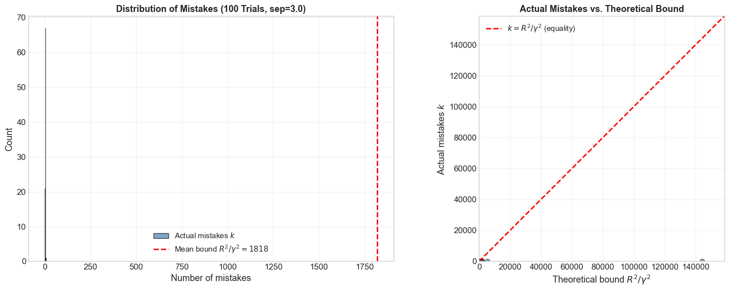
Summary over 100 trials (separation=3.0):
  Actual mistakes: mean=1.9, std=0.7, max=6, min=1
  Bound R^2/gamma^2: mean=1817.9, std=15006.1
  Fraction of bound used: mean=3.65%
  Bound is always respected: True
Observations#
The actual number of mistakes \(k\) is always at or below the theoretical bound \(R^2/\gamma^2\).
The bound is often loose – the actual number of mistakes is typically much smaller than the bound.
The bound is a worst-case guarantee, not an average-case prediction.
6.7 The Bound is Tight#
Despite appearing loose in practice, the bound \(k \leq R^2/\gamma^2\) is tight in the worst case. There exist datasets for which the perceptron makes exactly \(\lfloor R^2/\gamma^2 \rfloor\) mistakes.
Worst-Case Construction (Sketch)#
Consider the \(n\)-dimensional dataset consisting of the \(n\) standard basis vectors \(\mathbf{e}_1, \ldots, \mathbf{e}_n\), all labeled \(+1\). The separating direction is \(\mathbf{w}^* = \frac{1}{\sqrt{n}}(1, 1, \ldots, 1)\).
Margin: \(\gamma = \mathbf{w}^* \cdot \mathbf{e}_i = 1/\sqrt{n}\) for each \(i\).
Radius: \(R = \|\mathbf{e}_i\| = 1\).
Bound: \(R^2/\gamma^2 = 1/(1/n) = n\).
The perceptron, cycling through \(\mathbf{e}_1, \ldots, \mathbf{e}_n\) in order, needs to update on each one exactly once (each time adding a new basis direction), making exactly \(n\) mistakes. So the bound is achieved.
This shows the bound is asymptotically tight: there is no better general bound of the form \(C \cdot R^2/\gamma^2\) for some constant \(C < 1\).
6.8 Margin and Generalization#
The convergence theorem reveals a deep connection between geometric margin and learning complexity:
This means:
Larger margin \(\gamma\) \(\Rightarrow\) fewer mistakes \(\Rightarrow\) faster learning.
Smaller margin \(\Rightarrow\) more mistakes \(\Rightarrow\) harder problem.
This insight foreshadows one of the most important ideas in machine learning: the maximum margin principle.
Preview: Support Vector Machines#
While the perceptron finds any separating hyperplane, the Support Vector Machine (SVM) finds the one with the largest margin \(\gamma^*\). The motivation comes directly from the convergence theorem:
Among all separating hyperplanes, the one with the largest margin gives the tightest bound on the number of perceptron mistakes.
More importantly, larger margins correlate with better generalization (performance on unseen data).
The SVM was introduced by Vapnik and Chervonenkis (1963) and later developed into a practical algorithm by Boser, Guyon, and Vapnik (1992). The margin concept from the perceptron convergence theorem is at its theoretical core.
Connection to PAC Learning#
In the framework of Probably Approximately Correct (PAC) learning:
The ratio \(R/\gamma\) determines the effective complexity of the classification problem.
This ratio is related to the fat-shattering dimension, a generalization of the VC dimension for margin classifiers.
Sample complexity bounds for linear classifiers depend on \(R/\gamma\), not on the ambient dimension \(n\).
6.9 What Happens Without Separability?#
Show code cell source
import numpy as np
import matplotlib.pyplot as plt

# Generate NON-separable data: overlapping Gaussian clusters
np.random.seed(42)
n_per_class = 40

X0 = np.random.randn(n_per_class, 2) * 1.0 + np.array([-0.5, 0])
X1 = np.random.randn(n_per_class, 2) * 1.0 + np.array([0.5, 0])
X_nonsep = np.vstack([X0, X1])
y_nonsep = np.array([0] * n_per_class + [1] * n_per_class)

# Run perceptron for many epochs -- it should NOT converge
class PerceptronTracker:
    """Perceptron that tracks detailed history for non-separable data analysis."""

    def __init__(self, n_features, max_epochs=100):
        self.weights = np.zeros(n_features)
        self.bias = 0.0
        self.max_epochs = max_epochs
        self.errors_per_epoch = []
        self.accuracy_per_epoch = []

    def fit(self, X, y):
        X = np.atleast_2d(X)
        n_samples = X.shape[0]
        self.weights = np.zeros(X.shape[1])
        self.bias = 0.0
        self.errors_per_epoch = []
        self.accuracy_per_epoch = []

        for epoch in range(self.max_epochs):
            errors = 0
            for i in range(n_samples):
                y_hat = int(np.dot(self.weights, X[i]) + self.bias >= 0)
                if y_hat != y[i]:
                    update = (y[i] - y_hat)
                    self.weights += update * X[i]
                    self.bias += update
                    errors += 1

            self.errors_per_epoch.append(errors)
            self.accuracy_per_epoch.append(1 - errors / n_samples)

            if errors == 0:
                break

        return self


p_nonsep = PerceptronTracker(n_features=2, max_epochs=200)
p_nonsep.fit(X_nonsep, y_nonsep)

print(f"Epochs run: {len(p_nonsep.errors_per_epoch)}")
print(f"Converged: {p_nonsep.errors_per_epoch[-1] == 0}")
print(f"Errors in last 5 epochs: {p_nonsep.errors_per_epoch[-5:]}")
Epochs run: 200
Converged: False
Errors in last 5 epochs: [8, 8, 8, 8, 7]
Show code cell source
import numpy as np
import matplotlib.pyplot as plt

fig, axes = plt.subplots(1, 2, figsize=(16, 6))

# --- Panel 1: Errors per epoch (oscillating) ---
ax = axes[0]
epochs_range = range(1, len(p_nonsep.errors_per_epoch) + 1)
ax.plot(list(epochs_range), p_nonsep.errors_per_epoch, 'b-', linewidth=1, alpha=0.7)
ax.fill_between(list(epochs_range), p_nonsep.errors_per_epoch, alpha=0.15, color='red')
ax.axhline(y=0, color='green', linestyle='--', linewidth=1.5, alpha=0.5,
           label='Target: 0 errors')
ax.set_xlabel('Epoch', fontsize=13)
ax.set_ylabel('Errors per Epoch', fontsize=13)
ax.set_title('Non-Separable Data: Errors Oscillate Forever',
             fontsize=13, fontweight='bold', color='red')
ax.legend(fontsize=11)
ax.grid(True, alpha=0.3)

# --- Panel 2: Decision boundary at final epoch ---
ax = axes[1]

x_min, x_max = X_nonsep[:, 0].min() - 1, X_nonsep[:, 0].max() + 1
y_min, y_max = X_nonsep[:, 1].min() - 1, X_nonsep[:, 1].max() + 1
xx, yy = np.meshgrid(np.linspace(x_min, x_max, 200),
                     np.linspace(y_min, y_max, 200))
Z = xx * p_nonsep.weights[0] + yy * p_nonsep.weights[1] + p_nonsep.bias

ax.contourf(xx, yy, Z, levels=[-1e10, 0, 1e10],
            colors=['#FFCCCC', '#CCCCFF'], alpha=0.3)
ax.contour(xx, yy, Z, levels=[0], colors='black', linewidths=2)

ax.scatter(X_nonsep[y_nonsep == 0, 0], X_nonsep[y_nonsep == 0, 1],
           c='red', marker='o', s=40, edgecolors='black', alpha=0.7,
           label='Class 0')
ax.scatter(X_nonsep[y_nonsep == 1, 0], X_nonsep[y_nonsep == 1, 1],
           c='blue', marker='s', s=40, edgecolors='black', alpha=0.7,
           label='Class 1')

ax.set_xlabel('$x_1$', fontsize=13)
ax.set_ylabel('$x_2$', fontsize=13)
ax.set_title('Non-Separable Data: No Perfect Boundary Exists',
             fontsize=13, fontweight='bold', color='red')
ax.legend(fontsize=11)
ax.grid(True, alpha=0.3)

plt.tight_layout()
plt.show()
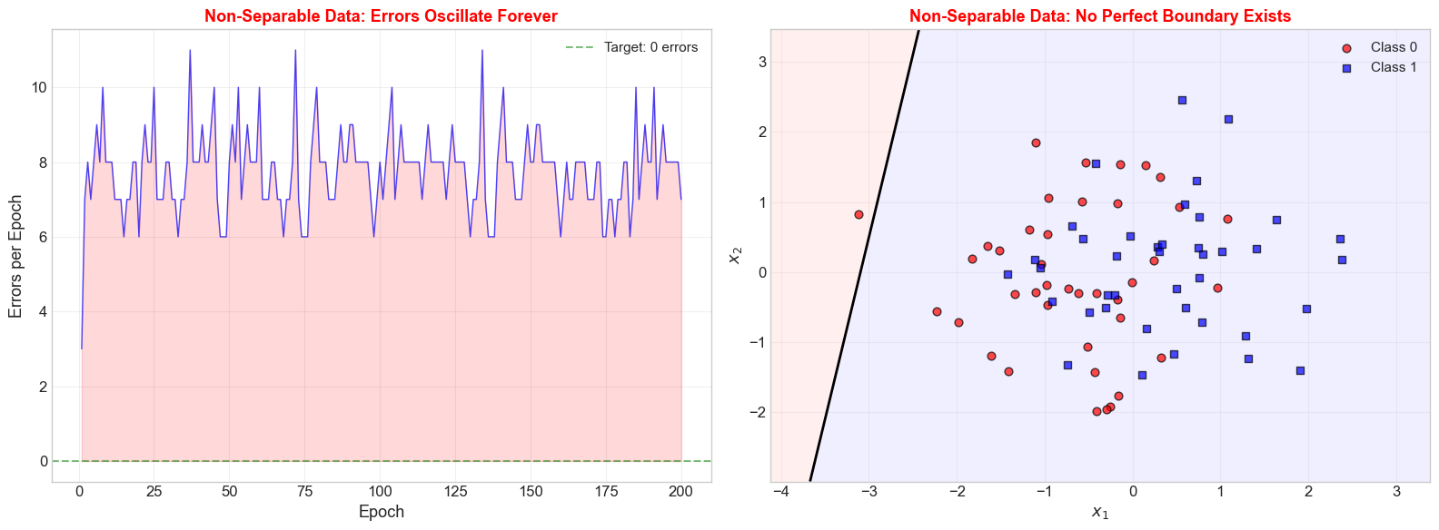
The Pocket Algorithm#
When data is not linearly separable, the standard perceptron never converges. The Pocket Algorithm (Gallant, 1990) is a simple modification:
Run the standard perceptron algorithm.
After each epoch, evaluate the current weights on the entire training set.
Keep a “pocket” copy of the best weights seen so far (the ones with the fewest errors).
Return the pocket weights when the algorithm terminates.
This gives an approximate solution that minimizes training error, even when perfect separation is impossible. It is a precursor to more sophisticated approaches like the relaxation algorithm and gradient descent on smooth loss functions.
6.10 Exercises#
Exercise 6.1: Compute R and gamma by Hand#
Consider the dataset (using \(\{-1, +1\}\) labels and the bias trick with \(x_0 = 1\)):
\(x_1\) |
\(x_2\) |
\(y\) |
Augmented: \((1, x_1, x_2)\) |
|---|---|---|---|
1 |
1 |
+1 |
(1, 1, 1) |
2 |
2 |
+1 |
(1, 2, 2) |
-1 |
-1 |
-1 |
(1, -1, -1) |
-2 |
0 |
-1 |
(1, -2, 0) |
Compute \(R = \max_i \|\tilde{\mathbf{x}}_i\|\) for the augmented vectors.
Find a separating unit vector \(\mathbf{w}^*\) and compute the margin \(\gamma = \min_i y_i(\mathbf{w}^* \cdot \tilde{\mathbf{x}}_i)\).
What is the convergence bound \(R^2/\gamma^2\)?
Run the perceptron by hand (or in code) and count the actual number of mistakes. Is it within the bound?
Exercise 6.2: Dimension Independence#
Prove that the bound \(k \leq R^2/\gamma^2\) does not explicitly depend on the dimensionality \(n\). That is, adding irrelevant features (columns of zeros) to the data does not change \(R\) or \(\gamma\).
Hint: If \(\tilde{\mathbf{x}}_i = (\mathbf{x}_i, 0, \ldots, 0)\) and \(\tilde{\mathbf{w}}^* = (\mathbf{w}^*, 0, \ldots, 0)\), compute \(\|\tilde{\mathbf{x}}_i\|\) and \(\tilde{\mathbf{w}}^* \cdot \tilde{\mathbf{x}}_i\).
Exercise 6.3: Achieving the Bound#
Consider the dataset in \(\mathbb{R}^n\) consisting of the \(n\) standard basis vectors \(\mathbf{e}_1, \ldots, \mathbf{e}_n\), all with label \(y = +1\).
What is \(R\)?
What is the optimal separating direction \(\mathbf{w}^*\) and the corresponding \(\gamma\)?
Show that \(R^2/\gamma^2 = n\).
Run the perceptron (presenting \(\mathbf{e}_1, \mathbf{e}_2, \ldots, \mathbf{e}_n\) in order). How many mistakes does it make? Does it match the bound?
Show code cell source
import numpy as np

# Exercise 6.3: Verification for the tight bound construction
print("=" * 60)
print("Exercise 6.3: Achieving the Bound")
print("=" * 60)

for n in [2, 3, 5, 10, 20, 50]:
    # n standard basis vectors, all labeled +1
    X_basis = np.eye(n)
    y_basis = np.ones(n)

    # Optimal w* = (1/sqrt(n), ..., 1/sqrt(n))
    w_star = np.ones(n) / np.sqrt(n)

    R = np.max(np.linalg.norm(X_basis, axis=1))  # = 1
    gamma = np.min(y_basis * (X_basis @ w_star))   # = 1/sqrt(n)
    bound = R**2 / gamma**2

    # Run perceptron ({-1,+1} convention: use +1 labels only)
    w = np.zeros(n)
    mistakes = 0
    for epoch in range(n + 5):
        no_errors = True
        for i in range(n):
            if w @ X_basis[i] <= 0:  # misclassification (should be > 0)
                w = w + X_basis[i]
                mistakes += 1
                no_errors = False
        if no_errors:
            break

    print(f"  n={n:>3d}: R={R:.1f}, gamma=1/sqrt({n})={gamma:.4f}, "
          f"bound={bound:.0f}, actual={mistakes}, "
          f"match={'YES' if mistakes == n else 'NO'}")
============================================================
Exercise 6.3: Achieving the Bound
============================================================
  n=  2: R=1.0, gamma=1/sqrt(2)=0.7071, bound=2, actual=2, match=YES
  n=  3: R=1.0, gamma=1/sqrt(3)=0.5774, bound=3, actual=3, match=YES
  n=  5: R=1.0, gamma=1/sqrt(5)=0.4472, bound=5, actual=5, match=YES
  n= 10: R=1.0, gamma=1/sqrt(10)=0.3162, bound=10, actual=10, match=YES
  n= 20: R=1.0, gamma=1/sqrt(20)=0.2236, bound=20, actual=20, match=YES
  n= 50: R=1.0, gamma=1/sqrt(50)=0.1414, bound=50, actual=50, match=YES