Chapter 33: Backpropagation Through Time

Chapter 33: Backpropagation Through Time#

In Chapter 16, we derived backpropagation for feedforward networks by applying the chain rule layer by layer. For recurrent networks, the same principle applies – but the chain extends through time. This temporal unrolling reveals a fundamental problem: gradients can vanish or explode exponentially.

The vanishing gradient problem, first identified by Hochreiter in his 1991 diploma thesis and formally analyzed by Bengio, Simard & Frasconi (1994), explains why simple RNNs fail to learn long-range dependencies. Understanding this failure is essential – it motivates the LSTM architecture that solved the problem and launched the modern era of sequence modeling.

In this chapter we derive the backpropagation through time (BPTT) algorithm, prove why gradients vanish or explode, demonstrate the failure empirically on a “remember the first character” task, and introduce two practical mitigations: gradient clipping and truncated BPTT.

Prerequisites

This chapter builds directly on Chapter 16 (backpropagation derivation) and Chapter 32 (simple RNN). Familiarity with matrix norms and eigenvalues is helpful but not strictly required.

Imports loaded: numpy, torch, matplotlib
PyTorch version: 2.7.0

33.1 Unrolling the RNN#

Recall the simple RNN equations from Chapter 32:

\[h_t = \tanh(W_h h_{t-1} + W_x x_t + b_h) \tag{RNN-1}\]

\[y_t = W_y h_t + b_y \tag{RNN-2}\]

When we process a sequence of length \(T\), the RNN applies these equations \(T\) times, with the same weights at each step. For the purpose of computing gradients, we can unroll the RNN into a feedforward network with \(T\) layers – one per time step.

Unrolling = Depth

An RNN processing a sequence of length \(T\) is equivalent, for gradient computation, to a feedforward network with \(T\) layers that share weights. A sequence of length 100 becomes a 100-layer deep network. The depth of this unrolled network is the source of the vanishing/exploding gradient problem.

At each time step \(t\), we may incur a loss \(\ell_t\) (e.g., cross-entropy between the predicted and actual next character). The total loss over the sequence is:

\[L = \sum_{t=1}^T \ell_t\]

../_images/1a631a208da04d2e63659f78cb3697967438fcd6d4e7d3cf82d428dabb2baec8.png

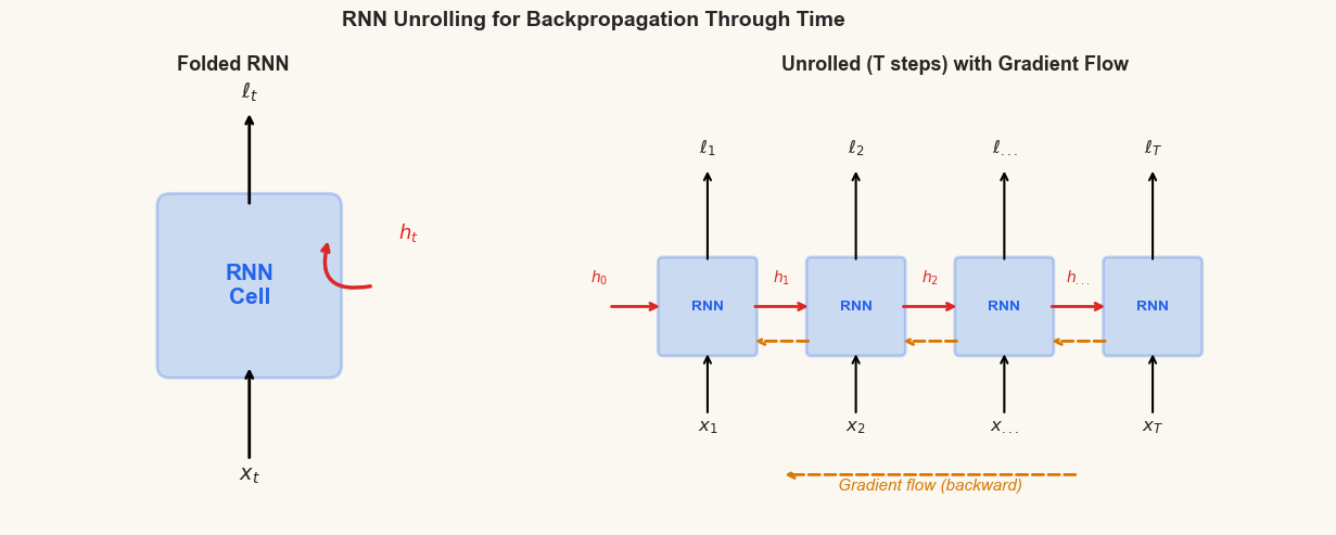
Each copy of the RNN cell shares the SAME weights.
Gradients flow backward through every time step (dashed arrows).
The longer the sequence, the deeper the effective network.

33.2 BPTT Derivation#

We now derive the backpropagation through time algorithm, extending the chain rule analysis of Chapter 16 to the temporal dimension.

Setup#

Let \(\ell_t\) be the loss at time step \(t\) (e.g., cross-entropy between the predicted next token and the ground truth). The total loss is \(L = \sum_{t=1}^T \ell_t\). We need the gradients \(\frac{\partial L}{\partial W_h}\), \(\frac{\partial L}{\partial W_x}\), and \(\frac{\partial L}{\partial b_h}\) to update the shared parameters.

The Chain Through Time#

Since \(W_h\) is used at every time step, its gradient accumulates contributions from all time steps:

\[\frac{\partial L}{\partial W_h} = \sum_{t=1}^T \frac{\partial \ell_t}{\partial W_h}\]

The loss \(\ell_t\) depends on \(W_h\) through the chain:

\[\ell_t \leftarrow y_t \leftarrow h_t \leftarrow h_{t-1} \leftarrow \cdots \leftarrow h_1 \leftarrow h_0\]

Applying the chain rule:

\[\frac{\partial \ell_t}{\partial W_h} = \sum_{k=1}^t \frac{\partial \ell_t}{\partial h_t} \underbrace{\left(\prod_{j=k+1}^t \frac{\partial h_j}{\partial h_{j-1}}\right)}_{\text{temporal Jacobian product}} \frac{\partial h_k}{\partial W_h}\]

Theorem (BPTT Gradient)

The gradient of the total loss with respect to the hidden-to-hidden weight matrix is:

\[\frac{\partial L}{\partial W_h} = \sum_{t=1}^T \sum_{k=1}^t \frac{\partial \ell_t}{\partial h_t} \left(\prod_{j=k+1}^t \frac{\partial h_j}{\partial h_{j-1}}\right) \frac{\partial h_k}{\partial W_h}\]

where the temporal Jacobian at each step is:

\[\frac{\partial h_j}{\partial h_{j-1}} = \text{diag}\left(1 - h_j^2\right) W_h\]

using the fact that \(\tanh'(z) = 1 - \tanh^2(z)\) and \(h_j = \tanh(W_h h_{j-1} + W_x x_j + b_h)\).

Connection to Chapter 16#

In Chapter 16, we derived four equations BP1–BP4 for feedforward networks. BPTT is the same chain rule, but applied to a network with shared weights across layers and multiple loss terms (one per time step):

Feedforward (Ch. 16)	Recurrent (BPTT)
One loss at the output	Loss at each time step
Different \(W^{(l)}\) per layer	Same \(W_h\) at every step
Chain through \(L\) layers	Chain through \(T\) time steps
\(\delta^{(l)} = \sigma'(z^{(l)}) \odot (W^{(l+1)})^\top \delta^{(l+1)}\)	\(\delta_t = (1 - h_t^2) \odot (W_h^\top \delta_{t+1} + \frac{\partial \ell_t}{\partial h_t})\)

BPTT Algorithm#

Algorithm: Backpropagation Through Time

Input: Sequence \(x_1, \ldots, x_T\); targets \(y_1^*, \ldots, y_T^*\); parameters \(W_x, W_h, W_y, b_h, b_y\).

Forward pass:

Set \(h_0 = \mathbf{0}\)
For \(t = 1, \ldots, T\):
- \(h_t = \tanh(W_h h_{t-1} + W_x x_t + b_h)\)
- \(y_t = W_y h_t + b_y\)
- Compute loss \(\ell_t = \text{Loss}(y_t, y_t^*)\)

Backward pass: 3. Initialize \(\delta_{T+1}^h = \mathbf{0}\) (no future gradient) 4. For \(t = T, T-1, \ldots, 1\):

\(\delta_t^y = \frac{\partial \ell_t}{\partial y_t}\) (output gradient)
\(\delta_t^h = W_y^\top \delta_t^y + W_h^\top \delta_{t+1}^h\) (total gradient at \(h_t\))
\(\delta_t^z = \delta_t^h \odot (1 - h_t^2)\) (through tanh)
Accumulate: \(\Delta W_h \mathrel{+}= \delta_t^z \, h_{t-1}^\top\)
Accumulate: \(\Delta W_x \mathrel{+}= \delta_t^z \, x_t^\top\)
Accumulate: \(\Delta b_h \mathrel{+}= \delta_t^z\)
Pass backward: \(\delta_t^h = \delta_t^z\) (for next iteration, used as \(\delta_{t+1}^h\)… but we already computed \(W_h^\top \delta_{t+1}^h\) above)

Update: \(W_h \leftarrow W_h - \eta \, \Delta W_h\), etc.

33.3 The Vanishing and Exploding Gradient Problem#

The BPTT formula contains the product of temporal Jacobians:

\[\prod_{j=k+1}^t \frac{\partial h_j}{\partial h_{j-1}} = \prod_{j=k+1}^t \text{diag}(1 - h_j^2) \, W_h\]

This is a product of \(t - k\) matrices. What happens to such a product as \(t - k\) grows large?

Theorem (Gradient Magnitude Bound)

Let \(\sigma_{\max}\) denote the largest singular value of \(W_h\), and let \(\gamma = \max_z |\tanh'(z)| = 1\). Then:

\[\left\|\prod_{j=k+1}^t \text{diag}(1 - h_j^2) \, W_h\right\| \le (\gamma \cdot \sigma_{\max})^{t-k}\]

Proof sketch. Each factor in the product has norm at most \(\|\text{diag}(1 - h_j^2)\| \cdot \|W_h\| \le \gamma \cdot \sigma_{\max}\). By sub-multiplicativity of the operator norm:

\[\left\|\prod_{j=k+1}^t A_j\right\| \le \prod_{j=k+1}^t \|A_j\| \le (\gamma \cdot \sigma_{\max})^{t-k}\]

Three regimes emerge:

Condition	Behavior	Consequence
\(\gamma \cdot \sigma_{\max} < 1\)	Gradients decay as \((\gamma \sigma_{\max})^{t-k}\)	Vanishing: early inputs are forgotten
\(\gamma \cdot \sigma_{\max} = 1\)	Gradients remain bounded	Ideal (but unstable equilibrium)
\(\gamma \cdot \sigma_{\max} > 1\)	Gradients grow as \((\gamma \sigma_{\max})^{t-k}\)	Exploding: training diverges

For \(\tanh\), \(\gamma = 1\), so the critical quantity is \(\sigma_{\max}(W_h)\). In practice, the diagonal factors \(\text{diag}(1 - h_j^2)\) have entries in \([0, 1]\), so even when \(\sigma_{\max}(W_h) = 1\), the gradient typically vanishes.

Historical Note

Hochreiter (1991) first identified the vanishing gradient problem in his diploma thesis (in German). Bengio, Simard & Frasconi (1994) published the first widely-read English analysis, proving that learning long-range dependencies with gradient descent is “difficult” – the gradient signal decays exponentially with the temporal distance. This paper is one of the most cited in all of deep learning.

Let us verify the theory numerically. We create a random \(W_h\) matrix and compute the product of Jacobians for increasing numbers of steps.

# Numerical verification: Jacobian product norms
np.random.seed(42)

hidden_size = 32

# Case 1: sigma_max(W_h) < 1 (vanishing)
W_h_small = np.random.randn(hidden_size, hidden_size) * 0.3
sigma_max_small = np.linalg.svd(W_h_small, compute_uv=False)[0]

# Case 2: sigma_max(W_h) > 1 (exploding)
W_h_large = np.random.randn(hidden_size, hidden_size) * 0.7
sigma_max_large = np.linalg.svd(W_h_large, compute_uv=False)[0]

print(f'Case 1 (vanishing): sigma_max = {sigma_max_small:.3f}')
print(f'Case 2 (exploding): sigma_max = {sigma_max_large:.3f}')
print()

# Compute ||product of Jacobians|| for T steps
T_max = 50
norms_small = []
norms_large = []

for T in range(1, T_max + 1):
    # Simulate: use random hidden states for the diagonal
    rng = np.random.default_rng(T)
    
    prod_small = np.eye(hidden_size)
    prod_large = np.eye(hidden_size)
    
    for j in range(T):
        # Random hidden state for tanh derivative
        h_j = np.tanh(rng.normal(0, 1, hidden_size))
        diag_j = np.diag(1 - h_j**2)
        
        prod_small = diag_j @ W_h_small @ prod_small
        prod_large = diag_j @ W_h_large @ prod_large
    
    norms_small.append(np.linalg.norm(prod_small))
    norms_large.append(np.linalg.norm(prod_large))

print(f'After {T_max} steps:')
print(f'  Vanishing case: ||Jacobian product|| = {norms_small[-1]:.2e}')
print(f'  Exploding case: ||Jacobian product|| = {norms_large[-1]:.2e}')

Case 1 (vanishing): sigma_max = 3.114
Case 2 (exploding): sigma_max = 7.628

After 50 steps:
  Vanishing case: ||Jacobian product|| = 1.46e+03
  Exploding case: ||Jacobian product|| = 2.49e+21

../_images/cb4835087f5fcfba82b581d2e4c7ed7e3d34a16ebf393794b301b59f89fff5de.png

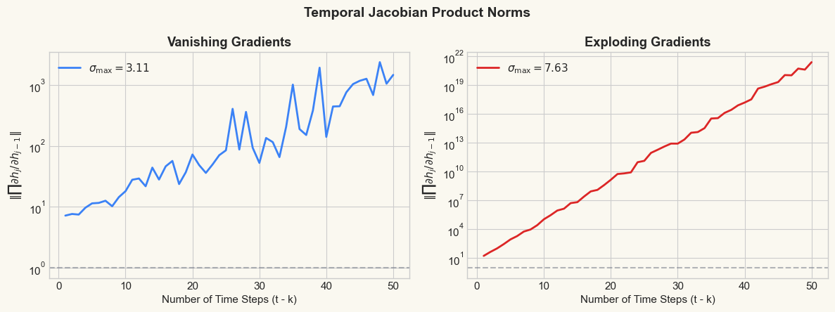
Left: gradients shrink exponentially -> network forgets distant inputs.
Right: gradients grow exponentially -> training becomes unstable.

33.4 Empirical Demonstration: The “Remember the First” Task#

To make the vanishing gradient problem tangible, we design a task that requires long-range memory: given a sequence of \(T\) random characters, the model must output the first character at the very end.

\[\underbrace{x_1}_{\text{remember this}}, \;x_2, \;x_3, \;\ldots, \;x_T \;\longrightarrow \;x_1\]

For this task, the gradient from the loss at time \(T\) must flow all the way back to time \(1\). If gradients vanish over \(T\) steps, the network cannot learn to solve this task.

We train a simple RNN with hidden_size=32 for 200 epochs on this task with varying sequence lengths \(T \in \{5, 10, 20, 50\}\).

# "Remember the first character" task

class RememberFirstRNN(nn.Module):
    """RNN that must predict the first character of a sequence at the end."""
    
    def __init__(self, vocab_size, hidden_size):
        super().__init__()
        self.hidden_size = hidden_size
        self.rnn = nn.RNN(vocab_size, hidden_size, batch_first=True)
        self.fc = nn.Linear(hidden_size, vocab_size)
    
    def forward(self, x):
        """x: (batch, seq_len, vocab_size) one-hot encoded.
        Returns logits for predicting the first character."""
        out, _ = self.rnn(x)         # (batch, seq_len, hidden_size)
        last_h = out[:, -1, :]       # (batch, hidden_size) -- final step
        logits = self.fc(last_h)     # (batch, vocab_size)
        return logits


def generate_remember_first_data(n_samples, seq_len, n_classes=8, seed=42):
    """Generate data for the 'remember the first' task.
    
    Returns
    -------
    X : tensor, shape (n_samples, seq_len, n_classes) -- one-hot
    y : tensor, shape (n_samples,) -- class of first character
    """
    rng = np.random.default_rng(seed)
    indices = rng.integers(0, n_classes, size=(n_samples, seq_len))
    X = torch.zeros(n_samples, seq_len, n_classes)
    for i in range(n_samples):
        for t in range(seq_len):
            X[i, t, indices[i, t]] = 1.0
    y = torch.tensor(indices[:, 0], dtype=torch.long)  # first character
    return X, y


print('RememberFirstRNN class and data generator defined.')
print('Task: given a sequence of T random characters, predict the first one.')

RememberFirstRNN class and data generator defined.
Task: given a sequence of T random characters, predict the first one.

# Train on different sequence lengths
seq_lengths = [5, 10, 20, 50]
n_classes = 8
hidden_size = 32
n_train = 512
n_test = 128
n_epochs = 200
batch_size = 64

results = {}  # seq_len -> {'losses': [...], 'accs': [...], 'grad_norms': [...]}

for seq_len in seq_lengths:
    torch.manual_seed(42)
    
    # Generate data
    X_train, y_train = generate_remember_first_data(n_train, seq_len, n_classes, seed=42)
    X_test, y_test = generate_remember_first_data(n_test, seq_len, n_classes, seed=99)
    
    # Create model
    model = RememberFirstRNN(n_classes, hidden_size)
    optimizer = torch.optim.Adam(model.parameters(), lr=0.005)
    loss_fn = nn.CrossEntropyLoss()
    
    losses = []
    accs = []
    grad_norms_wh = []
    
    for epoch in range(n_epochs):
        model.train()
        epoch_loss = 0.0
        n_batches = 0
        
        # Mini-batch training
        perm = torch.randperm(n_train)
        for start in range(0, n_train, batch_size):
            idx = perm[start:start+batch_size]
            xb = X_train[idx]
            yb = y_train[idx]
            
            logits = model(xb)
            loss = loss_fn(logits, yb)
            
            optimizer.zero_grad()
            loss.backward()
            
            # Record gradient norm of W_hh
            wh_grad = model.rnn.weight_hh_l0.grad
            if wh_grad is not None:
                grad_norms_wh.append(wh_grad.norm().item())
            
            optimizer.step()
            epoch_loss += loss.item()
            n_batches += 1
        
        losses.append(epoch_loss / n_batches)
        
        # Test accuracy
        model.eval()
        with torch.no_grad():
            test_logits = model(X_test)
            test_preds = test_logits.argmax(dim=1)
            acc = (test_preds == y_test).float().mean().item()
        accs.append(acc)
    
    results[seq_len] = {
        'losses': losses,
        'accs': accs,
        'grad_norms': grad_norms_wh
    }
    
    print(f'T={seq_len:3d}: final acc = {accs[-1]:.1%}, '
          f'final loss = {losses[-1]:.3f}, '
          f'chance = {1/n_classes:.1%}')

T=  5: final acc = 100.0%, final loss = 0.000, chance = 12.5%

T= 10: final acc = 100.0%, final loss = 0.001, chance = 12.5%

T= 20: final acc = 100.0%, final loss = 0.001, chance = 12.5%

T= 50: final acc = 10.2%, final loss = 0.451, chance = 12.5%

Show code cell source Hide code cell source

# Plot: accuracy vs sequence length and gradient norms
colors_seq = {5: BLUE, 10: GREEN, 20: AMBER, 50: RED}

fig, axes = plt.subplots(1, 3, figsize=(15, 4.5))

# Panel 1: Training loss
ax = axes[0]
for T in seq_lengths:
    ax.plot(results[T]['losses'], color=colors_seq[T], linewidth=1.5,
            label=f'T={T}')
ax.set_xlabel('Epoch')
ax.set_ylabel('Loss')
ax.set_title('Training Loss', fontweight='bold')
ax.legend()
chance_loss = -np.log(1/n_classes)
ax.axhline(y=chance_loss, color=GRAY, linestyle='--', alpha=0.5,
           label='Chance')

# Panel 2: Test accuracy
ax = axes[1]
for T in seq_lengths:
    ax.plot(results[T]['accs'], color=colors_seq[T], linewidth=1.5,
            label=f'T={T}')
ax.axhline(y=1/n_classes, color=GRAY, linestyle='--', alpha=0.5,
           label='Chance (12.5%)')
ax.set_xlabel('Epoch')
ax.set_ylabel('Accuracy')
ax.set_title('Test Accuracy', fontweight='bold')
ax.set_ylim(0, 1.05)
ax.legend()

# Panel 3: Final accuracy vs sequence length
ax = axes[2]
final_accs = [results[T]['accs'][-1] for T in seq_lengths]
bar_colors = [colors_seq[T] for T in seq_lengths]
bars = ax.bar([str(T) for T in seq_lengths], final_accs, color=bar_colors,
              edgecolor='white', linewidth=1.5)
ax.axhline(y=1/n_classes, color=GRAY, linestyle='--', alpha=0.5,
           label='Chance')
ax.set_xlabel('Sequence Length T')
ax.set_ylabel('Final Test Accuracy')
ax.set_title('Accuracy vs Sequence Length', fontweight='bold')
ax.set_ylim(0, 1.05)
for bar, acc in zip(bars, final_accs):
    ax.text(bar.get_x() + bar.get_width()/2, bar.get_height() + 0.02,
            f'{acc:.0%}', ha='center', va='bottom', fontweight='bold', fontsize=11)
ax.legend()

fig.suptitle('"Remember the First Character" Task: Simple RNN Performance',
             fontsize=14, fontweight='bold')
plt.tight_layout()
plt.show()

print('Short sequences (T=5, 10): RNN can learn to remember the first character.')
print('Long sequences (T=20, 50): accuracy collapses toward chance level.')
print('This is the vanishing gradient problem in action.')

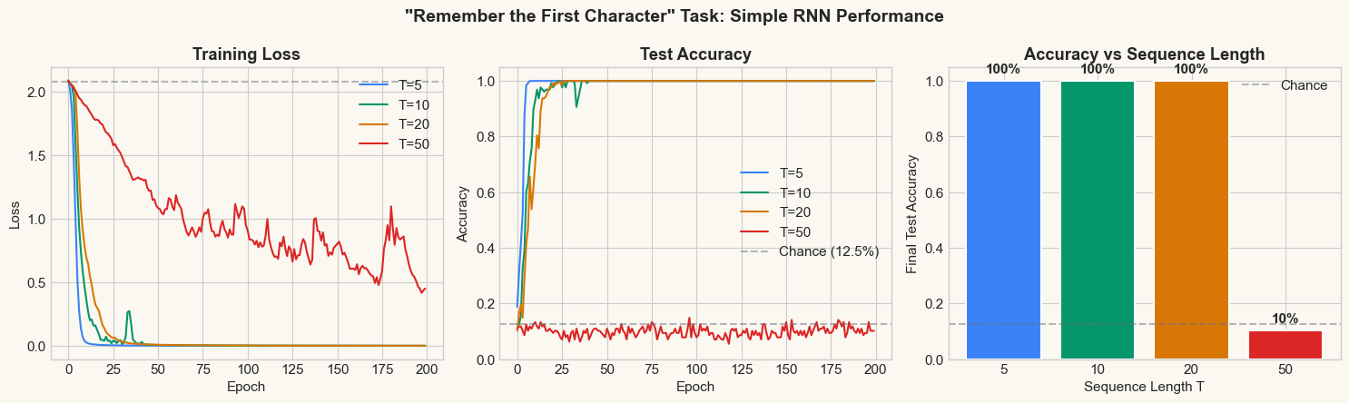
../_images/ab6761b0da14edb1661988ebcb5d4da7526092ad1ab5bab4cbdc29b578cbfee9.png

Short sequences (T=5, 10): RNN can learn to remember the first character.
Long sequences (T=20, 50): accuracy collapses toward chance level.
This is the vanishing gradient problem in action.

Show code cell source Hide code cell source

# Gradient norm at each time step (for a single example)
# We compute the gradient of the loss w.r.t. the hidden state at each step

torch.manual_seed(42)

fig, axes = plt.subplots(1, 2, figsize=(12, 4.5))

for plot_idx, seq_len in enumerate([10, 50]):
    model = RememberFirstRNN(n_classes, hidden_size)
    X_demo, y_demo = generate_remember_first_data(1, seq_len, n_classes, seed=42)
    
    # Manual forward pass to get hidden states with gradients
    x_input = X_demo  # (1, seq_len, n_classes)
    h = torch.zeros(1, 1, hidden_size)
    
    # Store hidden states
    hidden_states = []
    rnn_cell = model.rnn
    
    # Use the RNN layer step by step
    h_t = torch.zeros(1, 1, hidden_size, requires_grad=True)
    all_h = []
    
    # Forward through RNN step by step
    out, _ = model.rnn(x_input, h_t)
    last_h = out[:, -1, :]
    logits = model.fc(last_h)
    loss = nn.CrossEntropyLoss()(logits, y_demo)
    loss.backward()
    
    # Compute gradient norms at each time step using hooks
    # Alternative: compute numerically by looking at how much the loss changes
    # when we perturb h_t
    model2 = RememberFirstRNN(n_classes, hidden_size)
    # Copy weights
    model2.load_state_dict(model.state_dict())
    
    grad_norms_per_step = []
    
    for t_probe in range(seq_len):
        # Forward pass, but make hidden state at step t_probe require grad
        model2.eval()
        x_in = X_demo.clone()
        
        # Manually unroll to inject gradient tracking at step t_probe
        W_ih = model2.rnn.weight_ih_l0  # (hidden_size, input_size)
        W_hh = model2.rnn.weight_hh_l0  # (hidden_size, hidden_size)
        b_ih = model2.rnn.bias_ih_l0
        b_hh = model2.rnn.bias_hh_l0
        
        h_cur = torch.zeros(hidden_size)
        h_list = []
        
        for t in range(seq_len):
            x_t = x_in[0, t]  # (n_classes,)
            z = W_ih @ x_t + b_ih + W_hh @ h_cur + b_hh
            h_cur = torch.tanh(z)
            if t == t_probe:
                h_cur = h_cur.detach().requires_grad_(True)
                h_probe = h_cur
            h_list.append(h_cur)
        
        final_logits = model2.fc(h_list[-1].unsqueeze(0))
        probe_loss = nn.CrossEntropyLoss()(final_logits, y_demo)
        probe_loss.backward()
        
        grad_norm = h_probe.grad.norm().item()
        grad_norms_per_step.append(grad_norm)
    
    ax = axes[plot_idx]
    ax.semilogy(range(seq_len), grad_norms_per_step,
                color=BLUE if seq_len == 10 else RED,
                linewidth=2, marker='o', markersize=3)
    ax.set_xlabel('Time Step t')
    ax.set_ylabel('$\\|\\partial L / \\partial h_t\\|$ (log scale)')
    ax.set_title(f'Gradient Norm at Each Step (T={seq_len})',
                 fontweight='bold')
    ax.axvline(x=0, color=GREEN, linestyle='--', alpha=0.5, label='Target info (t=0)')
    ax.legend()

fig.suptitle('Gradient Signal Decay Through Time',
             fontsize=14, fontweight='bold')
plt.tight_layout()
plt.show()

print('The gradient at t=0 (where the target information resides) is much')
print('smaller than at t=T-1 (where the loss is computed).')
print('For T=50, the signal at t=0 is essentially zero -- the network')
print('cannot learn from the first character.')

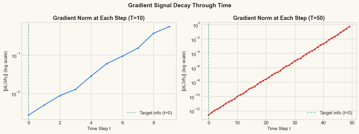
../_images/a8475213958e041df649ed5f5bb5e66454e99c716081ce345cad1c878b9e65f6.png

The gradient at t=0 (where the target information resides) is much
smaller than at t=T-1 (where the loss is computed).
For T=50, the signal at t=0 is essentially zero -- the network
cannot learn from the first character.

The Key Insight

The “remember the first character” experiment reveals the core failure mode of simple RNNs: the gradient signal from the loss at the end of the sequence decays exponentially as it propagates backward through time. For long sequences, the gradient at early time steps is effectively zero, making it impossible to learn dependencies that span many steps.

This is not a matter of training longer or using a better optimizer – it is a structural limitation of the simple RNN architecture. Overcoming it requires architectural changes (LSTM, GRU) that create alternative gradient pathways through the network.

33.5 Gradient Clipping#

While the vanishing gradient problem has no simple fix within the simple RNN architecture, the exploding gradient problem can be mitigated with a straightforward technique: gradient clipping.

The idea, introduced by Pascanu, Mikolov & Bengio (2013) in their paper “On the difficulty of training recurrent neural networks”, is to rescale the gradient whenever its norm exceeds a threshold \(\theta\):

\[\begin{split}\hat{g} = \begin{cases} \frac{\theta}{\|g\|} g & \text{if } \|g\| > \theta \\ g & \text{otherwise} \end{cases}\end{split}\]

In PyTorch, this is a single line:

torch.nn.utils.clip_grad_norm_(model.parameters(), max_norm=theta)

Clipping Prevents Explosion but Not Vanishing

Gradient clipping is a practical necessity for training RNNs, but it only addresses one half of the problem. It prevents gradients from exploding (causing NaN losses or wild parameter updates), but it does nothing to amplify gradients that have vanished. A clipped gradient of \(10^{-15}\) is still \(10^{-15}\).

Let us demonstrate gradient clipping on a sequence where the exploding gradient problem would otherwise cause training to diverge.

# Demonstrate gradient clipping
torch.manual_seed(42)

seq_len_clip = 20
X_clip, y_clip = generate_remember_first_data(256, seq_len_clip, n_classes, seed=42)

# Train with and without gradient clipping using a larger learning rate
# to provoke instability
configs = [
    ('No clipping', None, 0.01),
    ('Clip norm=5', 5.0, 0.01),
    ('Clip norm=1', 1.0, 0.01),
]

clip_results = {}

for name, clip_val, lr in configs:
    torch.manual_seed(42)
    model = RememberFirstRNN(n_classes, hidden_size)
    optimizer = torch.optim.SGD(model.parameters(), lr=lr)
    loss_fn = nn.CrossEntropyLoss()
    
    losses = []
    grad_norms = []
    
    for epoch in range(100):
        model.train()
        logits = model(X_clip)
        loss = loss_fn(logits, y_clip)
        
        optimizer.zero_grad()
        loss.backward()
        
        # Record gradient norm BEFORE clipping
        total_norm = 0.0
        for p in model.parameters():
            if p.grad is not None:
                total_norm += p.grad.data.norm(2).item() ** 2
        total_norm = total_norm ** 0.5
        grad_norms.append(total_norm)
        
        # Apply clipping if specified
        if clip_val is not None:
            torch.nn.utils.clip_grad_norm_(model.parameters(), max_norm=clip_val)
        
        optimizer.step()
        
        loss_val = loss.item()
        if np.isnan(loss_val) or np.isinf(loss_val):
            losses.append(float('nan'))
            # Fill remaining with NaN
            losses.extend([float('nan')] * (99 - epoch))
            grad_norms.extend([float('nan')] * (99 - epoch))
            break
        losses.append(loss_val)
    
    clip_results[name] = {'losses': losses, 'grad_norms': grad_norms}
    final_loss = losses[-1] if not np.isnan(losses[-1]) else 'DIVERGED'
    print(f'{name:20s}: final loss = {final_loss}')

No clipping         : final loss = 2.0764036178588867

Clip norm=5         : final loss = 2.0764036178588867

Clip norm=1         : final loss = 2.0764036178588867

../_images/aaac32765084d0a9c9f3b95f74950e43a879fb2dd294dfa0b6d9d03e5285c216.png

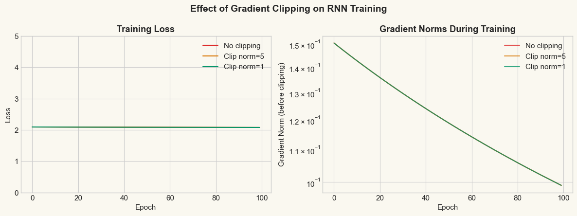
Gradient clipping prevents loss spikes and divergence.
However, it does NOT help the network learn long-range dependencies.
The vanishing gradient problem remains -- only explosion is tamed.

33.6 Truncated BPTT#

Full BPTT propagates gradients through the entire sequence of length \(T\). This has two costs:

Memory: We must store all \(T\) hidden states for the backward pass.
Time: The backward pass is \(O(T)\), which can be slow for long sequences.

Truncated backpropagation through time (TBPTT) addresses both costs by limiting the backward pass to only \(K\) steps, where \(K \ll T\).

How It Works#

Instead of backpropagating through the entire sequence:

Process the sequence in chunks of \(K\) time steps.
After each chunk, compute the loss and backpropagate through the \(K\) steps.
Detach the hidden state before starting the next chunk, severing the gradient connection to earlier time steps.

In PyTorch, detaching is a single operation: h = h.detach().

The Truncation Trade-off

Truncated BPTT trades long-range gradient flow for computational efficiency. With truncation length \(K\):

The network can still use long-range information (via the hidden state, which propagates forward without truncation).
But it can only learn from dependencies up to \(K\) steps apart (because gradients are cut beyond \(K\) steps).

Choosing \(K\) is an engineering judgment: too small and the network cannot learn medium-range patterns; too large and you lose the computational benefits (and still face vanishing gradients).

# Demonstrate truncated BPTT
def train_with_tbptt(model, X, y, K, n_epochs=100, lr=0.005):
    """Train an RNN using truncated BPTT with truncation length K.
    
    Parameters
    ----------
    model : RememberFirstRNN
    X : tensor (batch, seq_len, n_classes)
    y : tensor (batch,)
    K : int, truncation length (0 = full BPTT)
    """
    optimizer = torch.optim.Adam(model.parameters(), lr=lr)
    loss_fn = nn.CrossEntropyLoss()
    seq_len = X.shape[1]
    losses = []
    
    for epoch in range(n_epochs):
        model.train()
        
        if K == 0 or K >= seq_len:
            # Full BPTT
            logits = model(X)
            loss = loss_fn(logits, y)
            optimizer.zero_grad()
            loss.backward()
            torch.nn.utils.clip_grad_norm_(model.parameters(), max_norm=5.0)
            optimizer.step()
            losses.append(loss.item())
        else:
            # Truncated BPTT
            W_ih = model.rnn.weight_ih_l0
            W_hh = model.rnn.weight_hh_l0
            b_ih = model.rnn.bias_ih_l0
            b_hh = model.rnn.bias_hh_l0
            
            batch_size_local = X.shape[0]
            h = torch.zeros(batch_size_local, model.hidden_size)
            
            total_loss = 0.0
            steps_in_chunk = 0
            
            for t in range(seq_len):
                x_t = X[:, t, :]  # (batch, n_classes)
                z = x_t @ W_ih.t() + b_ih + h @ W_hh.t() + b_hh
                h = torch.tanh(z)
                steps_in_chunk += 1
                
                # At chunk boundaries (or end), detach
                if steps_in_chunk >= K and t < seq_len - 1:
                    h = h.detach()
                    steps_in_chunk = 0
            
            # Final prediction
            logits = model.fc(h)
            loss = loss_fn(logits, y)
            
            optimizer.zero_grad()
            loss.backward()
            torch.nn.utils.clip_grad_norm_(model.parameters(), max_norm=5.0)
            optimizer.step()
            losses.append(loss.item())
    
    return losses


# Compare full BPTT vs truncated on T=20 sequence
torch.manual_seed(42)
seq_len_tbptt = 20
X_tbptt, y_tbptt = generate_remember_first_data(256, seq_len_tbptt, n_classes, seed=42)
X_test_tbptt, y_test_tbptt = generate_remember_first_data(128, seq_len_tbptt, n_classes, seed=99)

tbptt_results = {}
truncation_lengths = [0, 20, 10, 5]  # 0 = full BPTT
labels_tbptt = ['Full BPTT', 'K=20 (full)', 'K=10', 'K=5']

for K, label in zip(truncation_lengths, labels_tbptt):
    torch.manual_seed(42)
    model = RememberFirstRNN(n_classes, hidden_size)
    losses = train_with_tbptt(model, X_tbptt, y_tbptt, K, n_epochs=150, lr=0.005)
    
    # Test accuracy
    model.eval()
    with torch.no_grad():
        test_logits = model(X_test_tbptt)
        acc = (test_logits.argmax(1) == y_test_tbptt).float().mean().item()
    
    tbptt_results[label] = {'losses': losses, 'acc': acc}
    print(f'{label:15s}: final acc = {acc:.1%}')

Full BPTT      : final acc = 99.2%

K=20 (full)    : final acc = 99.2%

K=10           : final acc = 20.3%

K=5            : final acc = 10.9%

../_images/a8b2a7118abd4d0886012add83226cb6ca45bfd8b94f28240f18e66eaf033631.png

Truncated BPTT with K < T cuts off gradient flow to early time steps.
For the "remember first" task, K=5 is too short -- the network cannot
learn to propagate information from step 0 to step 19.

In practice, truncated BPTT is used with K=20-200 to balance efficiency
and learning range. But for truly long-range dependencies, architectural
solutions (LSTM, Transformer) are needed.

Looking Ahead#

The vanishing gradient problem is not just a practical nuisance – it is a theoretical barrier that limits what simple RNNs can learn. Hochreiter and Schmidhuber recognized this in 1997 and proposed the Long Short-Term Memory (LSTM) architecture, which introduces gating mechanisms that create a “gradient highway” through time, allowing information to flow across hundreds of time steps without decay.

The LSTM is the subject of our next chapter. Understanding why it works requires understanding why the simple RNN fails – and that is precisely what we have established in this chapter:

Gradients are products of Jacobians along the time axis.
These products shrink (or grow) exponentially with sequence length.
Gradient clipping fixes explosion but not vanishing.
Truncated BPTT reduces cost but limits the learning horizon.

The LSTM’s solution is elegant: instead of multiplying by the same \(W_h\) at every step, it learns gates that control what to remember, what to forget, and what to output – creating a cell state that can carry information across arbitrary distances.

Exercises#

Exercise 33.1. Derive the BPTT gradient for \(W_x\) (the input-to-hidden weight matrix). Show that it has the same product-of-Jacobians structure as the gradient for \(W_h\), and explain why the vanishing gradient problem affects \(W_x\) equally.

Exercise 33.2. Consider a linear RNN (no activation function): \(h_t = W_h h_{t-1} + W_x x_t\). Show that the temporal Jacobian product simplifies to \(W_h^{t-k}\). If \(W_h\) has eigenvalues \(\lambda_1, \ldots, \lambda_n\), express the gradient in terms of \(\lambda_i^{t-k}\) and discuss when vanishing/exploding occurs.

Exercise 33.3. Run the “remember the first” experiment with hidden_size=128 instead of 32. Does increasing the hidden size help with the vanishing gradient problem? Why or why not?

Exercise 33.4. Implement BPTT manually for a 3-step RNN (without using loss.backward()). Given a concrete \(W_h\), \(W_x\), \(b_h\), input sequence \((x_1, x_2, x_3)\), and target \(y_3\):

Compute the forward pass.
Compute \(\frac{\partial L}{\partial W_h}\) by hand using the BPTT formula.
Verify your result against PyTorch’s autograd.

Exercise 33.5. Pascanu et al. (2013) also propose gradient norm rescaling as an alternative to clipping: instead of clipping to a maximum norm, rescale so the gradient always has a fixed norm \(\theta\). Implement this and compare training dynamics to standard clipping on the “remember the first” task with \(T=20\).