Chapter 30: DataLoaders, Training Loops, and Evaluation#
In the previous chapters, we assembled all the ingredients for training neural networks: loss functions that measure prediction quality (Chapter 26), optimizers that update parameters intelligently (Chapter 27), automatic differentiation that computes gradients effortlessly (Chapter 28), and PyTorch’s tensor abstractions that bring these pieces together at scale (Chapter 29).
Now we combine them into the training loop – the central algorithm of deep learning. Every neural network, from a 9-parameter XOR solver to a 175-billion-parameter GPT, is trained by the same iterative procedure: forward pass, loss computation, backward pass, parameter update. The details change; the structure does not.
This chapter makes the training loop explicit, introduces PyTorch’s data loading infrastructure, and applies everything to the MNIST handwritten digit recognition benchmark – the “hello world” of deep learning.
Show code cell source
import numpy as np
import matplotlib.pyplot as plt
import torch
import torch.nn as nn
import torch.optim as optim
from torch.utils.data import DataLoader, TensorDataset, random_split
import torchvision
import torchvision.transforms as transforms

# Consistent style for all plots
plt.rcParams.update({
    'figure.dpi': 100,
    'font.size': 11,
    'axes.titlesize': 13,
    'axes.labelsize': 12
})

# Standard color palette
BLUE = '#3b82f6'
GREEN = '#059669'
RED = '#dc2626'
AMBER = '#d97706'
INDIGO = '#4f46e5'

torch.manual_seed(42)
np.random.seed(42)

print('PyTorch version:', torch.__version__)
print('torchvision version:', torchvision.__version__)
PyTorch version: 2.7.0
torchvision version: 0.22.0
30.1 Training Loop Anatomy#
Every neural network training procedure follows the same pattern. We state it explicitly as an algorithm, mapping each step to the chapter where we derived the underlying mathematics.
Algorithm: The Standard Training Loop
Input: Model \(f_\theta\), training data \(\mathcal{D}\), loss function \(\mathcal{L}\), optimizer, number of epochs \(E\), batch size \(B\).
For epoch \(= 1, \ldots, E\):
Shuffle \(\mathcal{D}\) and partition into mini-batches of size \(B\).
For each mini-batch \((X_b, y_b)\):
Forward pass: Compute predictions \(\hat{y}_b = f_\theta(X_b)\). (Ch. 29)
Loss: Compute \(L = \mathcal{L}(\hat{y}_b, y_b)\). (Ch. 26)
Zero gradients: Set \(\nabla_\theta = 0\). (Ch. 28, 29)
Backward pass: Compute \(\nabla_\theta L\) via autograd. (Ch. 28)
Update: \(\theta \leftarrow \theta - \eta \cdot g(\nabla_\theta L)\) where \(g\) is the optimizer rule. (Ch. 27)
Evaluate on validation set (optional).
Return trained model \(f_\theta\).
In PyTorch, this translates directly into code:
# --- The canonical PyTorch training loop (pseudocode made concrete) ---

def train_one_epoch(model, dataloader, loss_fn, optimizer):
    """One pass through the entire training set."""
    model.train()                                # Set training mode
    total_loss = 0.0
    n_batches = 0

    for X_batch, y_batch in dataloader:           # Step 1.2: iterate mini-batches
        pred = model(X_batch)                     # Step 1.2.1: forward pass
        loss = loss_fn(pred, y_batch)             # Step 1.2.2: compute loss

        optimizer.zero_grad()                     # Step 1.2.3: zero gradients
        loss.backward()                           # Step 1.2.4: backward pass
        optimizer.step()                          # Step 1.2.5: update parameters

        total_loss += loss.item()
        n_batches += 1

    return total_loss / n_batches

print('train_one_epoch() defined -- maps directly to the algorithm above.')
print('Each line corresponds to a step we derived from first principles.')
train_one_epoch() defined -- maps directly to the algorithm above.
Each line corresponds to a step we derived from first principles.
30.2 Dataset and DataLoader#
Real datasets are too large to fit in a single tensor multiplication. PyTorch’s
torch.utils.data module provides two key abstractions:
Dataset: Stores samples and their labels. Implements__len__()and__getitem__().DataLoader: Wraps aDatasetto provide iteration, batching, shuffling, and parallel data loading.
Why Mini-Batches?
Recall from Chapter 27 that stochastic gradient descent uses a subset of the training data to estimate gradients. Mini-batches provide a favorable trade-off:
Batch size 1 (pure SGD): very noisy gradients, slow convergence.
Full batch (GD): exact gradients, but one step requires processing all data.
Mini-batch (typical: 32-256): gradient noise provides implicit regularization, and matrix operations are efficiently parallelized on modern hardware.
A Simple Example#
# --- DataLoader basics ---
from torch.utils.data import DataLoader, TensorDataset

# Create a toy dataset: 100 samples, 5 features
rng = np.random.default_rng(42)
X_toy = torch.randn(100, 5)
y_toy = (X_toy[:, 0] + X_toy[:, 1] > 0).long()  # binary classification

dataset = TensorDataset(X_toy, y_toy)
print(f'Dataset size: {len(dataset)}')
print(f'One sample: X.shape={dataset[0][0].shape}, y={dataset[0][1]}')

# DataLoader: batching + shuffling
loader = DataLoader(dataset, batch_size=16, shuffle=True)

print(f'\nNumber of batches: {len(loader)}')
for i, (X_b, y_b) in enumerate(loader):
    if i < 3:
        print(f'  Batch {i}: X.shape={X_b.shape}, y.shape={y_b.shape}')
    else:
        break
Dataset size: 100
One sample: X.shape=torch.Size([5]), y=1

Number of batches: 7
  Batch 0: X.shape=torch.Size([16, 5]), y.shape=torch.Size([16])
  Batch 1: X.shape=torch.Size([16, 5]), y.shape=torch.Size([16])
  Batch 2: X.shape=torch.Size([16, 5]), y.shape=torch.Size([16])
30.3 Loss Functions and Optimizers#
PyTorch implements all the loss functions and optimizers we derived in Chapters 26-27 as ready-to-use classes.
Loss Functions (Chapter 26 Revisited)#
PyTorch Class |
Mathematical Form |
Use Case |
|---|---|---|
|
\(\frac{1}{n}\sum(y_i - \hat{y}_i)^2\) |
Regression |
|
\(-\sum y_k \log \hat{y}_k\) |
Multi-class classification |
|
\(-[y\log\sigma(z) + (1-y)\log(1-\sigma(z))]\) |
Binary classification |
CrossEntropyLoss = LogSoftmax + NLLLoss
PyTorch’s nn.CrossEntropyLoss expects raw logits (unnormalized scores),
not probabilities. It internally applies log-softmax for numerical stability.
Do not apply softmax before CrossEntropyLoss – this is the most common
PyTorch beginner mistake.
Optimizers (Chapter 27 Revisited)#
PyTorch Class |
Algorithm |
Key Parameters |
|---|---|---|
|
(Stochastic) Gradient Descent |
|
|
Adaptive Moment Estimation |
|
|
Root Mean Square Propagation |
|
# --- Loss function demonstration ---
torch.manual_seed(42)

# CrossEntropyLoss expects raw logits, NOT probabilities
logits = torch.tensor([[2.0, 1.0, 0.1],    # sample 1: class 0 has highest score
                        [0.5, 2.5, 0.3]])   # sample 2: class 1 has highest score
targets = torch.tensor([0, 1])               # correct classes

ce_loss = nn.CrossEntropyLoss()
loss = ce_loss(logits, targets)
print(f'CrossEntropyLoss: {loss.item():.4f}')

# Manual verification (Chapter 26 formula)
import torch.nn.functional as F
log_probs = F.log_softmax(logits, dim=1)
manual_loss = -log_probs[0, 0] - log_probs[1, 1]  # negative log-prob of correct classes
manual_loss = manual_loss / 2  # mean over batch
print(f'Manual computation: {manual_loss.item():.4f}')
print(f'Match: {torch.isclose(loss, manual_loss).item()}')
CrossEntropyLoss: 0.3185
Manual computation: 0.3185
Match: True
30.4 MNIST MLP#
The MNIST dataset (LeCun et al., 1998) consists of 70,000 handwritten digit images, each \(28 \times 28\) pixels in grayscale. It is the standard benchmark for introducing neural network training on real data.
Historical Note
MNIST was created by Yann LeCun, Corinna Cortes, and Christopher J.C. Burges at AT&T Bell Labs. The dataset was derived from NIST Special Database 3 (Census Bureau employees) and Special Database 1 (high school students). LeCun used MNIST to demonstrate the effectiveness of convolutional networks in his landmark 1998 paper – we will replicate this in Chapter 31. For now, we use a simple multi-layer perceptron that treats each image as a flat 784-dimensional vector.
Loading the Data#
# --- Load MNIST ---
transform = transforms.Compose([
    transforms.ToTensor(),           # Convert PIL image to tensor [0, 1]
    transforms.Normalize((0.1307,), (0.3081,))  # MNIST mean and std
])

train_dataset = torchvision.datasets.MNIST(
    root='./data', train=True, download=True, transform=transform
)
test_dataset = torchvision.datasets.MNIST(
    root='./data', train=False, download=True, transform=transform
)

print(f'Training samples: {len(train_dataset)}')
print(f'Test samples:     {len(test_dataset)}')
print(f'Image shape:      {train_dataset[0][0].shape}')
print(f'Label example:    {train_dataset[0][1]}')
Training samples: 60000
Test samples:     10000
Image shape:      torch.Size([1, 28, 28])
Label example:    5
Show code cell source
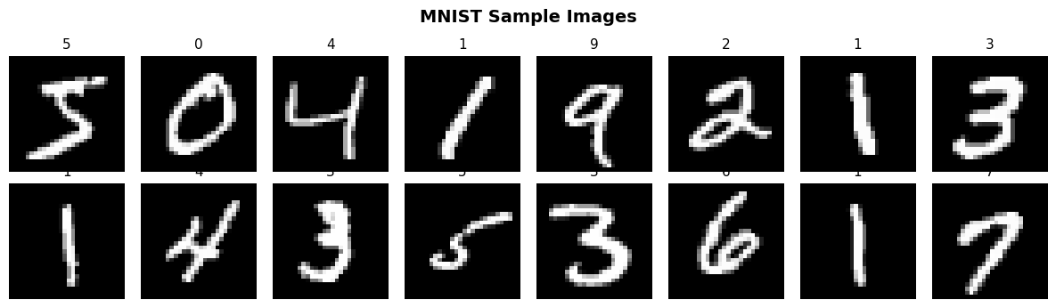
# --- Visualize sample digits ---
fig, axes = plt.subplots(2, 8, figsize=(12, 3.5))
for i, ax in enumerate(axes.flat):
    img, label = train_dataset[i]
    ax.imshow(img.squeeze(), cmap='gray')
    ax.set_title(str(label), fontsize=11)
    ax.axis('off')
fig.suptitle('MNIST Sample Images', fontsize=14, fontweight='bold')
plt.tight_layout()
plt.show()
# --- Create DataLoaders ---
train_loader = DataLoader(train_dataset, batch_size=64, shuffle=True)
test_loader = DataLoader(test_dataset, batch_size=64, shuffle=False)

print(f'Training batches per epoch: {len(train_loader)}')
print(f'Test batches: {len(test_loader)}')
Training batches per epoch: 938
Test batches: 157
Defining the MLP#
Our architecture: \(784 \to 128 \to 64 \to 10\). Each hidden layer uses ReLU activation (Chapter 17). The output layer produces raw logits for 10 classes.
# --- Define the MLP ---
class MNISTMLP(nn.Module):
    """Multi-layer perceptron for MNIST digit classification."""

    def __init__(self):
        super().__init__()
        self.flatten = nn.Flatten()          # (B, 1, 28, 28) -> (B, 784)
        self.layers = nn.Sequential(
            nn.Linear(784, 128),
            nn.ReLU(),
            nn.Linear(128, 64),
            nn.ReLU(),
            nn.Linear(64, 10),               # 10 classes, raw logits
        )

    def forward(self, x):
        x = self.flatten(x)
        return self.layers(x)

torch.manual_seed(42)
model = MNISTMLP()
print(model)

n_params = sum(p.numel() for p in model.parameters())
print(f'\nTotal trainable parameters: {n_params:,}')
MNISTMLP(
  (flatten): Flatten(start_dim=1, end_dim=-1)
  (layers): Sequential(
    (0): Linear(in_features=784, out_features=128, bias=True)
    (1): ReLU()
    (2): Linear(in_features=128, out_features=64, bias=True)
    (3): ReLU()
    (4): Linear(in_features=64, out_features=10, bias=True)
  )
)

Total trainable parameters: 109,386
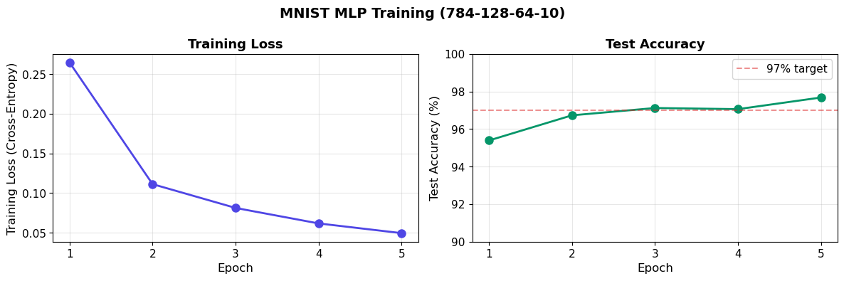
Training#
# --- Train the MLP ---
torch.manual_seed(42)
model = MNISTMLP()
loss_fn = nn.CrossEntropyLoss()
optimizer = optim.Adam(model.parameters(), lr=0.001)

train_losses = []
test_accuracies = []
n_epochs = 5

for epoch in range(n_epochs):
    # Training
    model.train()
    epoch_loss = 0.0
    n_batches = 0

    for X_batch, y_batch in train_loader:
        pred = model(X_batch)
        loss = loss_fn(pred, y_batch)

        optimizer.zero_grad()
        loss.backward()
        optimizer.step()

        epoch_loss += loss.item()
        n_batches += 1

    avg_loss = epoch_loss / n_batches
    train_losses.append(avg_loss)

    # Evaluation
    model.eval()
    correct = 0
    total = 0
    with torch.no_grad():
        for X_batch, y_batch in test_loader:
            pred = model(X_batch)
            _, predicted = torch.max(pred, 1)
            total += y_batch.size(0)
            correct += (predicted == y_batch).sum().item()

    accuracy = 100.0 * correct / total
    test_accuracies.append(accuracy)

    print(f'Epoch {epoch+1}/{n_epochs} -- '
          f'Train Loss: {avg_loss:.4f}, '
          f'Test Accuracy: {accuracy:.2f}%')

print(f'\nFinal test accuracy: {test_accuracies[-1]:.2f}%')
Epoch 1/5 -- Train Loss: 0.2645, Test Accuracy: 95.39%
Epoch 2/5 -- Train Loss: 0.1112, Test Accuracy: 96.73%
Epoch 3/5 -- Train Loss: 0.0812, Test Accuracy: 97.12%
Epoch 4/5 -- Train Loss: 0.0617, Test Accuracy: 97.06%
Epoch 5/5 -- Train Loss: 0.0494, Test Accuracy: 97.68%

Final test accuracy: 97.68%
Show code cell source
# --- Plot training curves ---
fig, (ax1, ax2) = plt.subplots(1, 2, figsize=(12, 4))

# Loss curve
ax1.plot(range(1, n_epochs + 1), train_losses, 'o-', color=INDIGO, linewidth=2, markersize=8)
ax1.set_xlabel('Epoch')
ax1.set_ylabel('Training Loss (Cross-Entropy)')
ax1.set_title('Training Loss', fontweight='bold')
ax1.grid(True, alpha=0.3)
ax1.set_xticks(range(1, n_epochs + 1))

# Accuracy curve
ax2.plot(range(1, n_epochs + 1), test_accuracies, 'o-', color=GREEN, linewidth=2, markersize=8)
ax2.set_xlabel('Epoch')
ax2.set_ylabel('Test Accuracy (%)')
ax2.set_title('Test Accuracy', fontweight='bold')
ax2.grid(True, alpha=0.3)
ax2.set_xticks(range(1, n_epochs + 1))
ax2.set_ylim(90, 100)
ax2.axhline(y=97, color=RED, linestyle='--', alpha=0.5, label='97% target')
ax2.legend()

fig.suptitle('MNIST MLP Training (784-128-64-10)', fontsize=14, fontweight='bold')
plt.tight_layout()
plt.show()
30.5 Evaluation Best Practices#
Proper evaluation requires care to avoid subtle bugs and misleading metrics.
model.train() vs. model.eval()#
Some layers behave differently during training and evaluation:
Dropout (Chapter 33, upcoming): randomly zeros activations during training, scales outputs during evaluation.
BatchNorm: uses batch statistics during training, running averages during evaluation.
Always call model.eval() before evaluation and model.train() before resuming training.
torch.no_grad()#
During evaluation, we do not need gradients. The torch.no_grad() context manager
disables gradient computation, saving memory and computation.
Common Mistake
Forgetting model.eval() or torch.no_grad() during evaluation does not cause
errors – it silently produces incorrect results (if the model uses dropout or
batchnorm) or wastes memory. Always use both.
Confusion Matrix#
A confusion matrix reveals per-class performance – essential for understanding which digits the model confuses.
# --- Compute confusion matrix ---
model.eval()
all_preds = []
all_labels = []

with torch.no_grad():
    for X_batch, y_batch in test_loader:
        pred = model(X_batch)
        _, predicted = torch.max(pred, 1)
        all_preds.extend(predicted.numpy())
        all_labels.extend(y_batch.numpy())

all_preds = np.array(all_preds)
all_labels = np.array(all_labels)

# Build confusion matrix manually (no sklearn dependency)
n_classes = 10
conf_matrix = np.zeros((n_classes, n_classes), dtype=int)
for true, pred in zip(all_labels, all_preds):
    conf_matrix[true, pred] += 1

# Per-class accuracy
print('Per-class accuracy:')
for digit in range(10):
    total = conf_matrix[digit].sum()
    correct = conf_matrix[digit, digit]
    print(f'  Digit {digit}: {correct}/{total} = {100*correct/total:.1f}%')
Per-class accuracy:
  Digit 0: 973/980 = 99.3%
  Digit 1: 1123/1135 = 98.9%
  Digit 2: 1012/1032 = 98.1%
  Digit 3: 998/1010 = 98.8%
  Digit 4: 954/982 = 97.1%
  Digit 5: 851/892 = 95.4%
  Digit 6: 936/958 = 97.7%
  Digit 7: 996/1028 = 96.9%
  Digit 8: 944/974 = 96.9%
  Digit 9: 981/1009 = 97.2%
Show code cell source
# --- Plot confusion matrix ---
fig, ax = plt.subplots(figsize=(8, 7))
im = ax.imshow(conf_matrix, interpolation='nearest', cmap='Blues')
ax.set_title('Confusion Matrix -- MNIST MLP', fontweight='bold', fontsize=14)
ax.set_xlabel('Predicted Label')
ax.set_ylabel('True Label')

# Add text annotations
thresh = conf_matrix.max() / 2.0
for i in range(n_classes):
    for j in range(n_classes):
        color = 'white' if conf_matrix[i, j] > thresh else 'black'
        ax.text(j, i, str(conf_matrix[i, j]),
                ha='center', va='center', color=color, fontsize=8)

ax.set_xticks(range(10))
ax.set_yticks(range(10))
fig.colorbar(im, ax=ax, fraction=0.046, pad=0.04)
plt.tight_layout()
plt.show()
Show code cell source
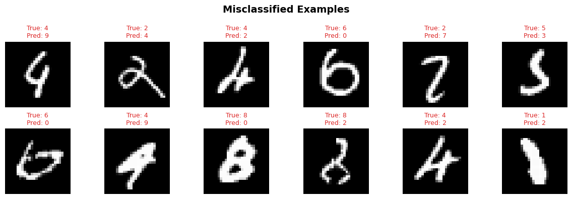
# --- Show some misclassified examples ---
misclassified_idx = np.where(all_preds != all_labels)[0]
n_show = min(12, len(misclassified_idx))

fig, axes = plt.subplots(2, 6, figsize=(12, 4))
for i, ax in enumerate(axes.flat[:n_show]):
    idx = misclassified_idx[i]
    img, _ = test_dataset[idx]
    ax.imshow(img.squeeze(), cmap='gray')
    ax.set_title(f'True: {all_labels[idx]}\nPred: {all_preds[idx]}',
                 fontsize=9, color=RED)
    ax.axis('off')

fig.suptitle('Misclassified Examples', fontsize=14, fontweight='bold')
plt.tight_layout()
plt.show()
Exercises#
Exercise 30.1. Modify the training loop to record the training loss per batch (not per epoch). Plot the loss curve for all batches across all 5 epochs. You should see a noisy but decreasing trend. How does this compare to the per-epoch curve?
Exercise 30.2. Replace optim.Adam with optim.SGD (lr=0.01, momentum=0.9)
and retrain the MNIST MLP. Compare the final accuracy and the shape of the loss
curve with the Adam version. Which optimizer converges faster in terms of epochs?
Exercise 30.3. Implement a validation split: use 50,000 samples for training
and 10,000 for validation (from the original 60,000 training set). Use
torch.utils.data.random_split(). Plot both training and validation loss curves
on the same axes. Do you observe any signs of overfitting?
Exercise 30.4. Experiment with the architecture: try (a) a single hidden layer with 256 units, (b) three hidden layers with 128-64-32 units, and © a very shallow network with one hidden layer of 32 units. Report the test accuracy for each. How does depth vs. width affect performance on MNIST?
Exercise 30.5. Add dropout (nn.Dropout(p=0.2)) after each ReLU in the MLP.
Train for 10 epochs instead of 5. Compare test accuracy with and without dropout.
Remember to verify that model.eval() disables dropout during evaluation.
References.
LeCun, Y., Bottou, L., Bengio, Y., and Haffner, P. (1998). “Gradient-Based Learning Applied to Document Recognition.” Proceedings of the IEEE, 86(11), 2278-2324.
Paszke, A., Gross, S., Massa, F., et al. (2019). “PyTorch: An Imperative Style, High-Performance Deep Learning Library.” NeurIPS 2019.
Kingma, D. P. and Ba, J. (2015). “Adam: A Method for Stochastic Optimization.” ICLR 2015.