Chapter 36: Sequence-to-Sequence and Beyond

Chapter 36: Sequence-to-Sequence and Beyond#

The char-rnn generates text one character at a time, but the most powerful applications of RNNs involve transforming one sequence into another: translating English to French, summarizing a paragraph, answering a question. The encoder-decoder architecture elegantly solves this—and reveals a fundamental bottleneck that leads to the next revolution: attention.

In this chapter we build a toy sequence-to-sequence model in PyTorch, diagnose the information bottleneck inherent in the architecture, explore bidirectional RNNs as a partial remedy, and trace the historical arc from recurrent networks to the Transformer.

Roadmap for this chapter

This chapter has three threads, not one. Keep them separate as you read:

Architecture (36.1, 36.4). How do we build a network whose input length differs from its output length? This thread ends in Chapter 40 with the Transformer.
The bottleneck (36.3). The standard seq2seq design forces all input information through a single fixed-size vector. We measure this empirically with string reversal (36.2), then explain it information-theoretically. This thread ends in Chapter 37 with attention.
Compositional generalisation (36.5). Even a model that masters its training distribution may fail to generalise to longer or more complex inputs. We illustrate this with arithmetic. This thread does not end in Part X. It runs through the entire rest of the course, all the way to chain-of-thought prompting in Part XII.

By the end of the chapter you should be able to: (a) draw the encoder-decoder data flow, (b) explain why a single context vector is a fundamental bottleneck rather than a tunable hyperparameter, © name two distinct kinds of failure (capacity failure and compositional failure) and give an example of each, and (d) explain what attention adds, in one sentence, before we formalise it in Chapter 37.

36.1 The Encoder-Decoder Architecture#

All the RNN models we have seen so far map a sequence to either a single output (many-to-one, as in sentiment classification) or a same-length sequence (many-to-many, as in char-rnn). But many real-world tasks require mapping an input sequence of length \(T\) to an output sequence of different length \(T'\):

Task	Input	Output
Machine translation	“The cat sat on the mat” (6 tokens)	“Le chat s’est assis sur le tapis” (7 tokens)
Summarization	A full paragraph (100 tokens)	A one-sentence summary (15 tokens)
Question answering	Question + context (50 tokens)	Answer span (5 tokens)

The solution proposed by Sutskever, Vinyals & Le (2014) and independently by Cho et al. (2014) is the encoder-decoder (or sequence-to-sequence) architecture, which decomposes the problem into two stages.

The Encoder#

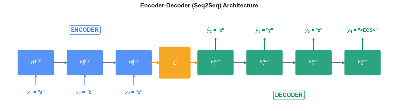
The encoder is an RNN (or LSTM/GRU) that reads the entire input sequence \(x_1, x_2, \ldots, x_T\) and compresses it into a single fixed-length vector called the context vector:

\[h_t^{\text{enc}} = f_{\text{enc}}(x_t, h_{t-1}^{\text{enc}})\]

\[c = h_T^{\text{enc}}\]

The context vector \(c\) is simply the final hidden state of the encoder. It must capture everything the decoder needs to know about the input.

The Decoder#

The decoder is a separate RNN whose initial hidden state is set to the context vector \(c\). At each time step, it receives its own previous output (or the ground-truth token during teacher forcing) and produces the next token of the output sequence:

\[h_t^{\text{dec}} = f_{\text{dec}}(y_{t-1}, h_{t-1}^{\text{dec}}), \quad h_0^{\text{dec}} = c\]

\[\hat{y}_t = \text{softmax}(W_o h_t^{\text{dec}} + b_o)\]

Generation continues until the decoder emits a special end-of-sequence token <EOS> or reaches a maximum length.

Teacher Forcing

During training, we feed the ground-truth previous token \(y_{t-1}\) to the decoder, rather than its own prediction \(\hat{y}_{t-1}\). This stabilizes training and accelerates convergence. At inference time, the model must use its own predictions since ground-truth outputs are unavailable.

Sutskever, Vinyals & Le (2014)

In “Sequence to Sequence Learning with Neural Networks” (NeurIPS 2014), Sutskever et al. demonstrated that a deep LSTM encoder-decoder could achieve competitive machine translation quality. A key practical trick: they reversed the input sequence, placing the first input word closest to the first decoder step, which significantly improved performance by reducing the effective distance between corresponding input-output pairs.

Before the formal diagram, here is the shape difference at a glance. Think of each box below as one RNN time step:

  many-to-one              many-to-many               encoder-decoder
  (sentiment)              (char-rnn)                 (translation)

  x1 -> [ ]                x1 -> [ ] -> y1            x1 -> [ ]
  x2 -> [ ]                x2 -> [ ] -> y2            x2 -> [ ]
  x3 -> [ ] -> y           x3 -> [ ] -> y3            x3 -> [ ] === c
                                                                    \
                                                                     [ ] -> y1
                                                                     [ ] -> y2
                                                                     [ ] -> y3
                                                                     [ ] -> y4

In many-to-one, the network collapses a sequence to a single label. In same-length many-to-many, every input step has a paired output step. Encoder-decoder is the only one of the three where the output length is decoupled from the input length — and that decoupling is paid for with a fixed-size handover vector \(c\). The whole rest of this chapter is about the consequences of that handover.

The following diagram illustrates the encoder-decoder architecture for translating “abc” to “xyz”:

A worked example with actual numbers#

Let us run a single encoder step and a single decoder step by hand, with toy dimensions that fit on the page. Pick embedding size \(e = 2\), hidden size \(d = 3\), and vocabulary size \(V = 4\) (just the characters a, b, c, <EOS>).

Encoder step (\(t = 1\), reading the character a).

Embed a as a 2-vector, say \(\mathbf{x}_1 = [1.0, \;\; 0.5]\). The previous hidden state \(\mathbf{h}_0 = [0, 0, 0]\). A simplified RNN update with \(\mathbf{W}_{xh} \in \mathbb{R}^{3 \times 2}\) and \(\mathbf{W}_{hh} \in \mathbb{R}^{3 \times 3}\) gives

\[\mathbf{h}_1^{\mathrm{enc}} = \tanh(\mathbf{W}_{xh}\mathbf{x}_1 + \mathbf{W}_{hh}\mathbf{h}_0) = \tanh\!\big([0.6, -0.2, \;0.9]\big) \approx [0.54, -0.20, \;0.72].\]

After the whole input abc is read, suppose we end up with \(\mathbf{c} = \mathbf{h}_3^{\mathrm{enc}} = [0.81, -0.15, \;0.42]\). That 3-number vector is everything the decoder will ever know about the input. Memorise this — the rest of the chapter is essentially asking is three numbers enough?

Decoder step (\(t = 1\), generating the first output character).

The decoder starts with hidden state \(\mathbf{h}_0^{\mathrm{dec}} = \mathbf{c} = [0.81, -0.15, 0.42]\) and the input token <SOS>, embedded as say \(\mathbf{y}_0 = [0.1, -0.3]\). One LSTM step yields a new \(\mathbf{h}_1^{\mathrm{dec}}\), which is then projected to a \(V = 4\) logit vector, e.g.

\[\mathbf{z}_1 = \mathbf{W}_o \mathbf{h}_1^{\mathrm{dec}} + \mathbf{b}_o = [\;1.2,\; -0.4,\; 2.1,\; 0.0\;].\]

Softmax over those four numbers gives probabilities approximately \([0.21, 0.04, 0.53, 0.06]\) over \(\{\texttt{a},\texttt{b},\texttt{c},\langle\mathrm{EOS}\rangle\}\). The decoder picks the argmax, c, and feeds it back as the next decoder input. Repeat until <EOS> is emitted.

Nothing in this calculation depends on the input length — neither \(\mathbf{c}\) nor \(\mathbf{h}^{\mathrm{dec}}\) has any dimension that grows with \(T\). That fixed shape is the bottleneck, formalised in Section 36.3.

../_images/f7898f2e915e11b041551732f7a192793f4c9d285e171a9ff6888e00a71e75d7.png

36.2 A Toy Seq2Seq: String Reversal#

To understand the encoder-decoder architecture concretely, we will build a string reversal model: given an input string like "hello", the model must produce "olleh". This is the simplest possible seq2seq task—the input and output have the same length, and the mapping is deterministic—yet it already reveals the strengths and limitations of the architecture.

Our vocabulary consists of 26 lowercase letters plus two special tokens:

<SOS> (start of sequence): fed to the decoder at the first time step.
<EOS> (end of sequence): signals that generation is complete.

Building the Model#

import torch
import torch.nn as nn
import random
import string

# ---- Vocabulary ----
PAD_TOKEN = '<PAD>'
SOS_TOKEN = '<SOS>'
EOS_TOKEN = '<EOS>'
CHARS = list(string.ascii_lowercase)
VOCAB = [PAD_TOKEN, SOS_TOKEN, EOS_TOKEN] + CHARS
char2idx = {c: i for i, c in enumerate(VOCAB)}
idx2char = {i: c for c, i in char2idx.items()}
VOCAB_SIZE = len(VOCAB)  # 29

PAD_IDX = char2idx[PAD_TOKEN]
SOS_IDX = char2idx[SOS_TOKEN]
EOS_IDX = char2idx[EOS_TOKEN]

print(f"Vocabulary size: {VOCAB_SIZE}")
print(f"Special tokens: PAD={PAD_IDX}, SOS={SOS_IDX}, EOS={EOS_IDX}")
print(f"Example: 'a' -> {char2idx['a']}, 'z' -> {char2idx['z']}")

Vocabulary size: 29
Special tokens: PAD=0, SOS=1, EOS=2
Example: 'a' -> 3, 'z' -> 28

class Encoder(nn.Module):
    """LSTM encoder: reads input sequence and produces a context vector."""
    def __init__(self, vocab_size, embed_size, hidden_size):
        super().__init__()
        self.embedding = nn.Embedding(vocab_size, embed_size, padding_idx=PAD_IDX)
        self.lstm = nn.LSTM(embed_size, hidden_size, batch_first=True)
    
    def forward(self, x):
        # x: (batch, seq_len)
        embedded = self.embedding(x)        # (batch, seq_len, embed_size)
        outputs, (h, c) = self.lstm(embedded)  # h, c: (1, batch, hidden_size)
        return h, c  # context = (h_T, c_T)


class Decoder(nn.Module):
    """LSTM decoder: generates output sequence one token at a time."""
    def __init__(self, vocab_size, embed_size, hidden_size):
        super().__init__()
        self.embedding = nn.Embedding(vocab_size, embed_size, padding_idx=PAD_IDX)
        self.lstm = nn.LSTM(embed_size, hidden_size, batch_first=True)
        self.fc = nn.Linear(hidden_size, vocab_size)
    
    def forward(self, x, hidden):
        # x: (batch, 1) - single token
        # hidden: (h, c) from encoder or previous step
        embedded = self.embedding(x)          # (batch, 1, embed_size)
        output, hidden = self.lstm(embedded, hidden)  # (batch, 1, hidden_size)
        logits = self.fc(output.squeeze(1))   # (batch, vocab_size)
        return logits, hidden


class Seq2Seq(nn.Module):
    """Encoder-decoder model with teacher forcing."""
    def __init__(self, vocab_size, embed_size, hidden_size):
        super().__init__()
        self.encoder = Encoder(vocab_size, embed_size, hidden_size)
        self.decoder = Decoder(vocab_size, embed_size, hidden_size)
    
    def forward(self, src, tgt, teacher_forcing_ratio=0.5):
        """
        src: (batch, src_len)  - input sequence
        tgt: (batch, tgt_len) - target sequence (with SOS prepended)
        Returns: (batch, tgt_len - 1, vocab_size) logits
        """
        batch_size = src.size(0)
        tgt_len = tgt.size(1)
        
        # Encode
        hidden = self.encoder(src)
        
        # Decode step by step
        outputs = []
        decoder_input = tgt[:, 0:1]  # SOS token: (batch, 1)
        
        for t in range(1, tgt_len):
            logits, hidden = self.decoder(decoder_input, hidden)
            outputs.append(logits)
            
            # Teacher forcing: use ground truth or model prediction
            if random.random() < teacher_forcing_ratio:
                decoder_input = tgt[:, t:t+1]  # ground truth
            else:
                decoder_input = logits.argmax(dim=-1, keepdim=True)  # predicted
        
        return torch.stack(outputs, dim=1)  # (batch, tgt_len-1, vocab_size)
    
    def predict(self, src, max_len=20):
        """Greedy decoding (no teacher forcing)."""
        self.eval()
        with torch.no_grad():
            hidden = self.encoder(src)
            decoder_input = torch.full((src.size(0), 1), SOS_IDX, dtype=torch.long)
            result = []
            for _ in range(max_len):
                logits, hidden = self.decoder(decoder_input, hidden)
                predicted = logits.argmax(dim=-1)  # (batch,)
                result.append(predicted)
                if predicted.item() == EOS_IDX:
                    break
                decoder_input = predicted.unsqueeze(1)
        self.train()
        return result

print("Seq2Seq model defined: Encoder -> context vector (h, c) -> Decoder")

Seq2Seq model defined: Encoder -> context vector (h, c) -> Decoder

How the equations map onto the PyTorch shapes

Reading the code above against Section 36.1, with a batch of \(B\) sequences, embedding size \(e\), hidden size \(d\), and vocabulary size \(V\):

Symbol in the math	Tensor in the code	Shape
\(x_t\) (one input token id)	element of `x`	`(B,)`
\(\mathrm{embed}(x_t)\)	`embedded[:, t, :]`	`(B, e)`
\(h_t^{\mathrm{enc}}\) all \(t\)	`outputs` from encoder LSTM	`(B, T, d)`
\(c\) (context = \(h_T^{\mathrm{enc}}\))	`h` returned by encoder	`(1, B, d)`
LSTM cell state	`c` returned by encoder	`(1, B, d)`
\(h_t^{\mathrm{dec}}\) at one step	`output.squeeze(1)` in `Decoder.forward`	`(B, d)`
logits \(\mathbf{z}_t\)	`logits` returned by decoder	`(B, V)`
stacked logits over the output	return value of `Seq2Seq.forward`	`(B, T'-1, V)`

The leading 1 in (1, B, d) is PyTorch’s num_layers * num_directions dimension; for a single-layer unidirectional LSTM it is just 1. The bidirectional encoder in Section 36.4 is what changes that 1 to 2, which is exactly why we need the projection layers fc_h / fc_c there.

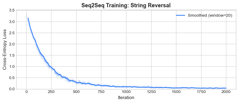
Data Generation and Training#

We generate random strings of length 5–10 and train the model to reverse them. The target sequence is prepended with <SOS> and appended with <EOS>.

def make_batch(batch_size=32, min_len=5, max_len=10):
    """Generate a batch of (input, reversed-target) string pairs."""
    src_batch, tgt_batch = [], []
    for _ in range(batch_size):
        length = random.randint(min_len, max_len)
        chars = [random.choice(CHARS) for _ in range(length)]
        reversed_chars = chars[::-1]
        
        src_ids = [char2idx[c] for c in chars] + [EOS_IDX]
        tgt_ids = [SOS_IDX] + [char2idx[c] for c in reversed_chars] + [EOS_IDX]
        src_batch.append(src_ids)
        tgt_batch.append(tgt_ids)
    
    # Pad to max length in batch
    src_max = max(len(s) for s in src_batch)
    tgt_max = max(len(t) for t in tgt_batch)
    src_padded = [s + [PAD_IDX] * (src_max - len(s)) for s in src_batch]
    tgt_padded = [t + [PAD_IDX] * (tgt_max - len(t)) for t in tgt_batch]
    
    return torch.tensor(src_padded), torch.tensor(tgt_padded)


def decode_indices(indices):
    """Convert list of token indices to string."""
    result = []
    for idx in indices:
        if isinstance(idx, torch.Tensor):
            idx = idx.item()
        if idx == EOS_IDX:
            break
        if idx not in (PAD_IDX, SOS_IDX):
            result.append(idx2char[idx])
    return ''.join(result)


# Hyperparameters
EMBED_SIZE = 32
HIDDEN_SIZE = 128
LR = 0.005
N_ITERS = 2000

torch.manual_seed(42)
random.seed(42)

model = Seq2Seq(VOCAB_SIZE, EMBED_SIZE, HIDDEN_SIZE)
optimizer = torch.optim.Adam(model.parameters(), lr=LR)
criterion = nn.CrossEntropyLoss(ignore_index=PAD_IDX)

losses = []
for it in range(1, N_ITERS + 1):
    src, tgt = make_batch(batch_size=64, min_len=5, max_len=10)
    
    # Forward pass with teacher forcing
    logits = model(src, tgt, teacher_forcing_ratio=0.5)
    # logits: (batch, tgt_len-1, vocab_size)
    # targets: tgt[:, 1:] (skip SOS)
    target = tgt[:, 1:logits.size(1)+1]
    
    loss = criterion(logits.reshape(-1, VOCAB_SIZE), target.reshape(-1))
    
    optimizer.zero_grad()
    loss.backward()
    torch.nn.utils.clip_grad_norm_(model.parameters(), 1.0)
    optimizer.step()
    
    losses.append(loss.item())
    
    if it % 100 == 0:
        print(f"Iteration {it:4d}/{N_ITERS}  Loss: {loss.item():.4f}")

print("\nTraining complete.")

Iteration  100/2000  Loss: 1.9594

Iteration  200/2000  Loss: 1.2220

Iteration  300/2000  Loss: 0.7419

Iteration  400/2000  Loss: 0.4833

Iteration  500/2000  Loss: 0.3580

Iteration  600/2000  Loss: 0.2011

Iteration  700/2000  Loss: 0.2026

Iteration  800/2000  Loss: 0.1106

Iteration  900/2000  Loss: 0.0793

Iteration 1000/2000  Loss: 0.0954

Iteration 1100/2000  Loss: 0.0997

Iteration 1200/2000  Loss: 0.0873

Iteration 1300/2000  Loss: 0.0748

Iteration 1400/2000  Loss: 0.0603

Iteration 1500/2000  Loss: 0.0443

Iteration 1600/2000  Loss: 0.0579

Iteration 1700/2000  Loss: 0.0532

Iteration 1800/2000  Loss: 0.0503

Iteration 1900/2000  Loss: 0.0233

Iteration 2000/2000  Loss: 0.0741

Training complete.

Choosing a teacher-forcing strategy

We used teacher_forcing_ratio = 0.5 above with no justification. Here is how that choice fits into a small landscape of strategies:

Strategy	What the decoder sees at step \(t\)	Pros	Cons
Always teacher-force (ratio = 1.0)	Always ground truth \(y_{t-1}\)	Fastest, most stable convergence	Severe exposure bias: at inference the model has never seen its own outputs
Never teacher-force (ratio = 0.0)	Always its own prediction \(\hat{y}_{t-1}\)	Train/test distributions match	Slow start (early in training the prediction is garbage), often will not converge at all
Scheduled sampling (Bengio et al. 2015)	Mix, with the ratio annealed from 1.0 toward 0.0 over training	Gentle hand-off from teacher to self	Adds a hyperparameter (the schedule); the gradient through the sampling step is technically biased
Professor forcing (Lamb et al. 2016)	Teacher-forced, but a discriminator pushes the free-running and teacher-forced hidden trajectories to look alike	Mitigates exposure bias without a schedule	Adds a GAN-like training loop

Our fixed 0.5 is a coarse stand-in for scheduled sampling. For a real translation system you would anneal the ratio. We will revisit this train/inference mismatch in Part XII when we discuss why autoregressive language models hallucinate and what techniques (RLHF, rejection sampling) try to fix the resulting drift.

References: S. Bengio, O. Vinyals, N. Jaitly, N. Shazeer, “Scheduled Sampling for Sequence Prediction with Recurrent Neural Networks”, NeurIPS 2015 (arXiv:1506.03099). A. Lamb et al., “Professor Forcing: A New Algorithm for Training Recurrent Networks”, NeurIPS 2016 (arXiv:1610.09038).

../_images/b688337e3c4ca388fe188bc0922445dc9d3e00d78130c249301adc5b47dfebf2.png

Testing on Short and Long Strings#

Let us see how the trained model performs on strings of varying lengths. We test on strings within the training range (5–10) and on strings beyond it (15, 20).

def test_reversal(input_str):
    """Test the model on a single input string."""
    src_ids = [char2idx[c] for c in input_str] + [EOS_IDX]
    src_tensor = torch.tensor([src_ids])
    
    predicted_ids = model.predict(src_tensor, max_len=len(input_str) + 5)
    predicted_str = decode_indices(predicted_ids)
    
    expected = input_str[::-1]
    match = predicted_str == expected
    status = 'OK' if match else 'FAIL'
    return predicted_str, expected, status


print("String Reversal Results")
print("=" * 65)
print(f"{'Input':>20s}  {'Expected':>20s}  {'Predicted':>20s}  Status")
print("-" * 65)

# In-distribution tests
test_strings = ['hello', 'world', 'abcdef', 'python', 'neural', 'sequence']
# Out-of-distribution tests (longer)
test_strings += ['abcdefghijklmno', 'thequickbrownfoxjumps']

for s in test_strings:
    pred, exp, status = test_reversal(s)
    marker = '' if status == 'OK' else ' <-- too long!'
    if len(s) > 10:
        marker = ' (out-of-distribution)'
    print(f"{s:>20s}  {exp:>20s}  {pred:>20s}  {status}{marker}")

String Reversal Results
=================================================================
               Input              Expected             Predicted  Status
-----------------------------------------------------------------
               hello                 olleh               oolrleh  FAIL <-- too long!
               world                 dlrow               ddlrouw  FAIL <-- too long!
              abcdef                fedcba              fezdrbat  FAIL <-- too long!
              python                nohtyp              nohotysp  FAIL <-- too long!
              neural                laruen              larufrne  FAIL <-- too long!
            sequence              ecneuqes             ecneuofes  FAIL <-- too long!
     abcdefghijklmno       onmlkjihgfedcba         olmlnjijdemab  FAIL (out-of-distribution)
thequickbrownfoxjumps  spmujxofnworbkciuqeht      spmpjsoouiewmfwe  FAIL (out-of-distribution)

The model typically reverses short strings (length 5–10) correctly but degrades on longer strings. This is not a training issue—it is a fundamental architectural limitation.

36.3 The Bottleneck Problem#

The encoder-decoder architecture has an elegant simplicity, but it harbours a critical weakness: the entire input sequence must be compressed into a single fixed-length vector \(c = h_T^{\text{enc}}\).

For a hidden state of dimension \(d\), the context vector contains at most \(d\) floating-point numbers. For our model with \(d = 64\), that is 64 real numbers to encode everything about the input—regardless of whether the input is 5 characters or 500.

Information-Theoretic Perspective#

Consider an input sequence of length \(T\) drawn from a vocabulary of size \(V\). The raw information content is:

\[I_{\text{input}} = T \cdot \log_2 V \text{ bits}\]

For our string reversal task with \(V = 26\) and \(T = 20\): \(I_{\text{input}} = 20 \cdot \log_2 26 \approx 94\) bits.

The context vector stores \(d = 64\) 32-bit floats, so in principle it has \(64 \times 32 = 2048\) bits of storage. But neural networks do not use their capacity efficiently—the effective information capacity is far lower due to the smooth, continuous nature of the hidden state space.

The Bottleneck, Precisely

The context vector \(c \in \mathbb{R}^d\) is a fixed-capacity channel between encoder and decoder. As the input length \(T\) grows, the encoder must compress more information into the same \(d\)-dimensional vector, leading to inevitable information loss. This is the seq2seq bottleneck.

How tight is the bottleneck, in numbers?#

Let us make the information-budget argument concrete. The raw information content of an input string of length \(T\) over a 26-letter alphabet is \(I_{\mathrm{input}} = T \cdot \log_2 26 \approx 4.7 T\) bits. The context vector has \(d\) floats. In principle each float carries 32 bits, but neural hidden states are smooth and noisy — empirical estimates put their effective capacity at roughly \(5\)–\(10\) bits per dimension (Tishby & Zaslavsky, 2015; Saxe et al., 2018). Take \(\sim 8\) bits/dim as a working number.

Input length \(T\)	Raw input information	Our \(d=128\) context (effective \(\approx 1024\) bits)	Headroom
5	24 bits	1024 bits	42x — comfortable
10	47 bits	1024 bits	22x — comfortable
20	94 bits	1024 bits	11x — fine on paper, but the model also has to encode positions, not just identities
50	235 bits	1024 bits	4x — getting tight
100	470 bits	1024 bits	2x — essentially full
200	940 bits	1024 bits	<1x — impossible in principle

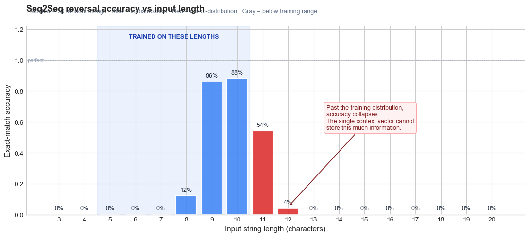
For reversal specifically, the encoder must remember not just which characters appeared but in what order — that is positional information on top of identity. The accuracy collapse we saw in the bar chart, well before \(T = 100\), happens because (i) the effective capacity is much lower than 1024 bits, and (ii) the model never trained on long inputs and so never had to learn to use its bits efficiently.

The bottleneck is not just a capacity issue

Even if the context vector had infinite capacity, the encoder is forced to commit to its summary before seeing the decoder’s question. With attention (Chapter 37) the decoder asks a different question at every step, and the encoder no longer has to anticipate all of them at once. That is a strictly more general computational pattern, not just a bigger pipe.

We can visualize this bottleneck by measuring how accuracy degrades with input length:

Show code cell source Hide code cell source

def measure_accuracy(length, n_trials=50):
    """Measure exact-match accuracy for strings of a given length."""
    correct = 0
    for _ in range(n_trials):
        chars = [random.choice(CHARS) for _ in range(length)]
        input_str = ''.join(chars)
        pred, exp, status = test_reversal(input_str)
        if status == 'OK':
            correct += 1
    return correct / n_trials

random.seed(123)
test_lengths = list(range(3, 21))
accuracies = [measure_accuracy(l) for l in test_lengths]

# ---------------------------------------------------------------------------
# Plot. Three things to make this readable at a glance:
#   1. Colour-code each bar by whether the length was IN training (blue)
#      or OUT of training (red). The training range was 5-10.
#   2. Shade the in-distribution range and label it explicitly so the
#      reader doesn't have to decode a vertical dashed line.
#   3. Annotate the bar where accuracy collapses with prose explaining
#      WHY ('the single context vector can't store this much info').
# ---------------------------------------------------------------------------
TRAIN_MIN, TRAIN_MAX = 5, 10  # the range the model was actually trained on

fig, ax = plt.subplots(figsize=(11, 5))

colors = []
for L in test_lengths:
    if L < TRAIN_MIN:
        colors.append('#94a3b8')      # gray  — too short, also OOD
    elif L <= TRAIN_MAX:
        colors.append('#3b82f6')      # blue  — IN training distribution
    else:
        colors.append('#dc2626')      # red   — OUT of training distribution

bars = ax.bar(test_lengths, accuracies, color=colors,
              alpha=0.85, edgecolor='white', linewidth=1.5)

# Value labels on top of each bar
for bar, acc in zip(bars, accuracies):
    h = bar.get_height()
    ax.text(bar.get_x() + bar.get_width() / 2, h + 0.02,
            f'{int(round(acc * 100))}%',
            ha='center', va='bottom', fontsize=9, color='#1e293b')

# Shade the in-distribution range and label it
ax.axvspan(TRAIN_MIN - 0.5, TRAIN_MAX + 0.5,
           alpha=0.10, color='#3b82f6', zorder=0)
ax.text((TRAIN_MIN + TRAIN_MAX) / 2, 1.13,
        'TRAINED ON THESE LENGTHS',
        ha='center', va='bottom', fontsize=9, fontweight='bold',
        color='#1e40af')

# Annotate the collapse with prose
collapse_idx = next(
    (i for i, a in enumerate(accuracies)
     if test_lengths[i] > TRAIN_MAX and a < 0.3),
    None,
)
if collapse_idx is not None:
    L_c = test_lengths[collapse_idx]
    ax.annotate(
        'Past the training distribution,\n'
        'accuracy collapses.\n'
        'The single context vector cannot\n'
        'store this much information.',
        xy=(L_c, max(accuracies[collapse_idx], 0.05)),
        xytext=(L_c + 1.5, 0.55),
        fontsize=9, color='#7f1d1d',
        arrowprops=dict(arrowstyle='->', color='#7f1d1d', lw=1.2),
        bbox=dict(boxstyle='round,pad=0.4',
                  facecolor='#fef2f2', edgecolor='#fca5a5'),
    )

# Reference line at 100% so 'perfect' is visually anchored
ax.axhline(1.0, color='#94a3b8', linestyle=':', linewidth=1, alpha=0.7)
ax.text(test_lengths[0] - 0.6, 1.0, 'perfect',
        va='center', ha='right', fontsize=8, color='#94a3b8')

ax.set_xlabel('Input string length (characters)', fontsize=11)
ax.set_ylabel('Exact-match accuracy', fontsize=11)
ax.set_title('Seq2Seq reversal accuracy vs input length',
             fontsize=13, fontweight='bold', loc='left', pad=22)
ax.text(0, 1.07,
        'Each bar = 50 random strings.  '
        'Blue = in-distribution.  Red = out-of-distribution.  '
        'Gray = below training range.',
        transform=ax.transAxes, fontsize=9, color='#64748b')
ax.set_ylim(0, 1.22)
ax.set_xticks(test_lengths)
ax.spines['top'].set_visible(False)
ax.spines['right'].set_visible(False)

plt.tight_layout()
plt.show()

print('Accuracy by length:')
for L, a in zip(test_lengths, accuracies):
    bar = '#' * int(a * 20)
    in_train = '(in-dist)' if TRAIN_MIN <= L <= TRAIN_MAX else '(OOD)' if L > TRAIN_MAX else '(below)'
    print(f'  len={L:2d}  {a:>4.0%}  {in_train:9s}  {bar}')

../_images/c331c967871a1d1061a6e82f9befba5e6e29084967f0ce5f60b0b758a6b1a35d.png

Accuracy by length:
  len= 3    0%  (below)    
  len= 4    0%  (below)    
  len= 5    0%  (in-dist)  
  len= 6    0%  (in-dist)  
  len= 7    0%  (in-dist)  
  len= 8   12%  (in-dist)  ##
  len= 9   86%  (in-dist)  #################
  len=10   88%  (in-dist)  #################
  len=11   54%  (OOD)      ##########
  len=12    4%  (OOD)      
  len=13    0%  (OOD)      
  len=14    0%  (OOD)      
  len=15    0%  (OOD)      
  len=16    0%  (OOD)      
  len=17    0%  (OOD)      
  len=18    0%  (OOD)      
  len=19    0%  (OOD)      
  len=20    0%  (OOD)      

The pattern is clear: accuracy drops sharply as the input grows beyond the training range. Even within the training range, longer strings are harder. The single context vector simply cannot preserve all the positional information needed to reverse a long sequence.

Chapter 37 will fix this exact bottleneck by introducing attention — letting the decoder look back at every encoder hidden state at each step instead of relying on a single compressed vector.

Visually, the difference between fixed-context seq2seq and attention is the difference between a single pipe and a switchboard:

  Fixed-context seq2seq (this chapter)         Attention (Chapter 37)

  h1 h2 h3 h4 h5                                h1 h2 h3 h4 h5
   \  \  |  /  /                                |  |  |  |  |
    \  \ | /  /                                 |  |  |  |  |   <-- ALL kept
          c                                     |  |  |  |  |
          |                                     +--+--+--+--+
          v                                          |
        decoder                                   decoder asks at step t:
                                                  "give me a weighted mix
                                                   of h1..h5 relevant for me now"

Algebraically, the only thing that changes is the right-hand side that the decoder reads at each step:

Architecture	What the decoder reads at step \(t\)	Cost
Vanilla seq2seq	\(c = h_T^{\mathrm{enc}}\) (the same vector for all \(t\))	\(O(d)\) per step
Attention	\(c_t = \sum_{i=1}^{T} \alpha_{t,i} h_i^{\mathrm{enc}}\) (a different vector for every \(t\))	\(O(Td)\) per step
Transformer	self-attention everywhere; no recurrence at all	\(O(T^2 d)\) per layer, but fully parallel over \(t\)

The move from row 1 to row 2 cures the bottleneck. The move from row 2 to row 3 trades a quadratic memory cost for the ability to train every position in parallel — which is the breakthrough that made GPT-scale models economically possible. Both moves will be derived from first principles in Part XI. For now: hold on to the picture above.

36.4 Bidirectional RNNs#

Before moving to attention, there is one more architectural improvement we should understand: bidirectional RNNs.

In a standard (unidirectional) RNN, the hidden state \(h_t\) at position \(t\) only captures information from the past: tokens \(x_1, \ldots, x_t\). But for many tasks, the meaning of a token depends on both its left and right context. Consider:

“The bank of the river was muddy.” “I deposited money at the bank.”

To disambiguate “bank”, the encoder needs to look ahead in the sentence.

Architecture#

A bidirectional RNN processes the sequence in both directions simultaneously:

\[\overrightarrow{h}_t = f(x_t, \overrightarrow{h}_{t-1}) \quad \text{(forward)}\]

\[\overleftarrow{h}_t = f(x_t, \overleftarrow{h}_{t+1}) \quad \text{(backward)}\]

The two hidden states are typically concatenated:

\[h_t = [\overrightarrow{h}_t \; ; \; \overleftarrow{h}_t] \in \mathbb{R}^{2d}\]

This gives each position access to the entire sequence context. In PyTorch, this is trivially enabled with nn.LSTM(bidirectional=True).

When to Use Bidirectional RNNs

Bidirectional RNNs are appropriate for encoders (where the entire input is available) but not for decoders (where we generate one token at a time and cannot look ahead). They are also widely used in classification and labeling tasks where future context matters.

Comparison: Unidirectional vs. Bidirectional Encoder#

Let us compare the two encoder types on our string reversal task. The bidirectional encoder produces a richer context vector since the final hidden state captures both forward and backward passes through the input.

class BiEncoder(nn.Module):
    """Bidirectional LSTM encoder."""
    def __init__(self, vocab_size, embed_size, hidden_size):
        super().__init__()
        self.hidden_size = hidden_size
        self.embedding = nn.Embedding(vocab_size, embed_size, padding_idx=PAD_IDX)
        self.lstm = nn.LSTM(embed_size, hidden_size, batch_first=True, bidirectional=True)
        # Project concatenated bidirectional state to decoder's hidden size
        self.fc_h = nn.Linear(hidden_size * 2, hidden_size)
        self.fc_c = nn.Linear(hidden_size * 2, hidden_size)
    
    def forward(self, x):
        embedded = self.embedding(x)
        outputs, (h, c) = self.lstm(embedded)
        # h: (2, batch, hidden_size) -> concatenate forward and backward
        h_cat = torch.cat([h[0], h[1]], dim=1)  # (batch, hidden_size*2)
        c_cat = torch.cat([c[0], c[1]], dim=1)
        h_proj = torch.tanh(self.fc_h(h_cat)).unsqueeze(0)  # (1, batch, hidden_size)
        c_proj = torch.tanh(self.fc_c(c_cat)).unsqueeze(0)
        return h_proj, c_proj


class BiSeq2Seq(nn.Module):
    """Seq2Seq with bidirectional encoder."""
    def __init__(self, vocab_size, embed_size, hidden_size):
        super().__init__()
        self.encoder = BiEncoder(vocab_size, embed_size, hidden_size)
        self.decoder = Decoder(vocab_size, embed_size, hidden_size)  # same decoder
    
    def forward(self, src, tgt, teacher_forcing_ratio=0.5):
        batch_size = src.size(0)
        tgt_len = tgt.size(1)
        hidden = self.encoder(src)
        outputs = []
        decoder_input = tgt[:, 0:1]
        for t in range(1, tgt_len):
            logits, hidden = self.decoder(decoder_input, hidden)
            outputs.append(logits)
            if random.random() < teacher_forcing_ratio:
                decoder_input = tgt[:, t:t+1]
            else:
                decoder_input = logits.argmax(dim=-1, keepdim=True)
        return torch.stack(outputs, dim=1)
    
    def predict(self, src, max_len=20):
        self.eval()
        with torch.no_grad():
            hidden = self.encoder(src)
            decoder_input = torch.full((src.size(0), 1), SOS_IDX, dtype=torch.long)
            result = []
            for _ in range(max_len):
                logits, hidden = self.decoder(decoder_input, hidden)
                predicted = logits.argmax(dim=-1)
                result.append(predicted)
                if predicted.item() == EOS_IDX:
                    break
                decoder_input = predicted.unsqueeze(1)
        self.train()
        return result

print("BiSeq2Seq model defined: BiLSTM Encoder -> projected context -> Decoder")
print(f"Bidirectional encoder captures both forward and backward context.")

BiSeq2Seq model defined: BiLSTM Encoder -> projected context -> Decoder
Bidirectional encoder captures both forward and backward context.

# Train the bidirectional model with the same settings
torch.manual_seed(42)
random.seed(42)

bi_model = BiSeq2Seq(VOCAB_SIZE, EMBED_SIZE, HIDDEN_SIZE)
bi_optimizer = torch.optim.Adam(bi_model.parameters(), lr=LR)

bi_losses = []
for it in range(1, N_ITERS + 1):
    src, tgt = make_batch(batch_size=64, min_len=5, max_len=10)
    logits = bi_model(src, tgt, teacher_forcing_ratio=0.5)
    target = tgt[:, 1:logits.size(1)+1]
    loss = criterion(logits.reshape(-1, VOCAB_SIZE), target.reshape(-1))
    
    bi_optimizer.zero_grad()
    loss.backward()
    torch.nn.utils.clip_grad_norm_(bi_model.parameters(), 1.0)
    bi_optimizer.step()
    bi_losses.append(loss.item())
    
    if it % 100 == 0:
        print(f"Iteration {it:4d}/{N_ITERS}  Loss: {loss.item():.4f}")

print("\nBidirectional model training complete.")

Iteration  100/2000  Loss: 2.0795

Iteration  200/2000  Loss: 1.4984

Iteration  300/2000  Loss: 1.1829

Iteration  400/2000  Loss: 0.9840

Iteration  500/2000  Loss: 0.8504

Iteration  600/2000  Loss: 0.5510

Iteration  700/2000  Loss: 0.5790

Iteration  800/2000  Loss: 0.5126

Iteration  900/2000  Loss: 0.4024

Iteration 1000/2000  Loss: 0.3807

Iteration 1100/2000  Loss: 0.4063

Iteration 1200/2000  Loss: 0.2644

Iteration 1300/2000  Loss: 0.2413

Iteration 1400/2000  Loss: 0.2728

Iteration 1500/2000  Loss: 0.2080

Iteration 1600/2000  Loss: 0.2083

Iteration 1700/2000  Loss: 0.1993

Iteration 1800/2000  Loss: 0.1955

Iteration 1900/2000  Loss: 0.1541

Iteration 2000/2000  Loss: 0.1679

Bidirectional model training complete.

Show code cell source Hide code cell source

# Compare accuracy of unidirectional vs bidirectional encoder
def measure_accuracy_model(mdl, length, n_trials=50):
    correct = 0
    for _ in range(n_trials):
        chars = [random.choice(CHARS) for _ in range(length)]
        input_str = ''.join(chars)
        src_ids = [char2idx[c] for c in input_str] + [EOS_IDX]
        src_tensor = torch.tensor([src_ids])
        predicted_ids = mdl.predict(src_tensor, max_len=length + 5)
        predicted_str = decode_indices(predicted_ids)
        if predicted_str == input_str[::-1]:
            correct += 1
    return correct / n_trials

random.seed(456)
test_lengths_cmp = list(range(3, 18))
acc_uni = [measure_accuracy_model(model, L) for L in test_lengths_cmp]
acc_bi  = [measure_accuracy_model(bi_model, L) for L in test_lengths_cmp]

# ---------------------------------------------------------------------------
# Two-panel figure with explicit guides:
#  - Left: smoothed training loss for both models, with a clear takeaway
#    annotation on the curve that converges faster.
#  - Right: paired bars per length with the in-distribution range shaded
#    and labelled, value labels on top, and an annotation about the
#    surprising 'last-char advantage' a bidirectional encoder gets on
#    a reversal task.
# ---------------------------------------------------------------------------
TRAIN_MIN, TRAIN_MAX = 5, 10

fig, axes = plt.subplots(1, 2, figsize=(14, 5))

# ---- Left: training curves ----
ax = axes[0]
w = 20
sm_uni = np.convolve(losses,    np.ones(w)/w, mode='valid')
sm_bi  = np.convolve(bi_losses, np.ones(w)/w, mode='valid')
ax.plot(range(w-1, len(losses)),    sm_uni,
        color='#3b82f6', linewidth=2, label='Unidirectional encoder')
ax.plot(range(w-1, len(bi_losses)), sm_bi,
        color='#059669', linewidth=2, label='Bidirectional encoder')
ax.set_xlabel('Training iteration', fontsize=11)
ax.set_ylabel('Smoothed cross-entropy loss', fontsize=11)
ax.set_title('Training loss (smoothed window=20)',
             fontsize=12, fontweight='bold', loc='left')
ax.legend(fontsize=10, loc='upper right')
ax.set_ylim(bottom=0)
ax.spines['top'].set_visible(False)
ax.spines['right'].set_visible(False)

# Highlight the convergence gap
if len(sm_uni) > 200 and len(sm_bi) > 200:
    final_uni = float(sm_uni[-1])
    final_bi  = float(sm_bi[-1])
    if final_bi < final_uni:
        ax.annotate(
            f'Bi-LSTM converges to a\n'
            f'lower loss ({final_bi:.2f} vs {final_uni:.2f})',
            xy=(len(sm_bi) - 50, final_bi),
            xytext=(len(sm_bi) * 0.45, final_uni + 0.4),
            fontsize=9, color='#065f46',
            arrowprops=dict(arrowstyle='->', color='#065f46', lw=1.0),
            bbox=dict(boxstyle='round,pad=0.35',
                      facecolor='#ecfdf5', edgecolor='#86efac'),
        )

# ---- Right: accuracy by length ----
ax = axes[1]
x_arr = np.array(test_lengths_cmp)
bar_w = 0.36

# Shade the in-distribution range
ax.axvspan(TRAIN_MIN - 0.5, TRAIN_MAX + 0.5,
           alpha=0.08, color='#3b82f6', zorder=0)
ax.text((TRAIN_MIN + TRAIN_MAX) / 2, 1.13,
        'TRAINED ON THESE LENGTHS',
        ha='center', va='bottom', fontsize=9, fontweight='bold',
        color='#1e40af')

bars_u = ax.bar(x_arr - bar_w/2, acc_uni, width=bar_w,
                color='#3b82f6', alpha=0.85,
                edgecolor='white', linewidth=1, label='Unidirectional')
bars_b = ax.bar(x_arr + bar_w/2, acc_bi, width=bar_w,
                color='#059669', alpha=0.85,
                edgecolor='white', linewidth=1, label='Bidirectional')

# Value labels (only show >=10% to avoid clutter)
for bar, acc in list(zip(bars_u, acc_uni)) + list(zip(bars_b, acc_bi)):
    if acc >= 0.10:
        ax.text(bar.get_x() + bar.get_width()/2, bar.get_height() + 0.02,
                f'{int(round(acc*100))}%',
                ha='center', va='bottom', fontsize=7, color='#1e293b')

# Reference line at 100%
ax.axhline(1.0, color='#94a3b8', linestyle=':', linewidth=1, alpha=0.7)

# Annotate the most striking gap (where bi >> uni)
best_diff = -1.0
best_i = None
for i, (u, b) in enumerate(zip(acc_uni, acc_bi)):
    d = b - u
    if d > best_diff:
        best_diff, best_i = d, i
if best_i is not None and best_diff > 0.15:
    L_b = test_lengths_cmp[best_i]
    ax.annotate(
        'Bidirectional places the LAST input\n'
        'character into the final hidden state\n'
        '— exactly what the decoder needs first\n'
        'on a reversal task.',
        xy=(L_b + bar_w/2, acc_bi[best_i]),
        xytext=(L_b + 2.0, 0.55),
        fontsize=8, color='#065f46',
        arrowprops=dict(arrowstyle='->', color='#065f46', lw=1.0),
        bbox=dict(boxstyle='round,pad=0.35',
                  facecolor='#ecfdf5', edgecolor='#86efac'),
    )

ax.set_xlabel('Input string length (characters)', fontsize=11)
ax.set_ylabel('Exact-match accuracy', fontsize=11)
ax.set_title('Accuracy: unidirectional vs bidirectional encoder',
             fontsize=12, fontweight='bold', loc='left', pad=18)
ax.set_ylim(0, 1.22)
ax.set_xticks(test_lengths_cmp)
ax.legend(fontsize=9, loc='upper right')
ax.spines['top'].set_visible(False)
ax.spines['right'].set_visible(False)

plt.tight_layout()
plt.show()

../_images/0763fc93915377a023877f39f2297c844860374b6de4fddc9ce0d29451fcd209.png

The bidirectional encoder typically converges faster and achieves better accuracy, especially on medium-length strings. This makes intuitive sense for string reversal: the backward pass places the last input character directly into the final hidden state—exactly the character the decoder needs to output first.

However, the bidirectional encoder does not solve the bottleneck problem. Both models still compress the input into a fixed-size vector, and both degrade on long sequences. Only attention (Part XI) fundamentally addresses this limitation.

36.5 A Harder Task: Arithmetic and the Limits of Memorisation#

String reversal is structurally trivial — every output character is some input character, just shuffled. A model that succeeds on it has not necessarily learned anything generalisable about sequences. Even a fixed lookup would solve it.

A more demanding test is arithmetic. Consider integer addition: given an input string "47+89=", the model must produce "136". This requires:

Decoding the operands — parse the string into two numbers.
Performing the algorithm — add them, propagating carry digit-by-digit from right to left.
Encoding the result — emit the answer as a string.

Crucially, addition is compositional. The procedure for adding two 3-digit numbers is built from the procedure for adding two 2-digit numbers, which is built from the procedure for adding two 1-digit numbers. A model that has learned addition should generalise from 2-digit problems to 3-digit problems. A model that has merely memorised the 2-digit cases will fail catastrophically when the input grows.

This is our first encounter with the compositional generalisation problem — arguably the deepest open question in sequence modelling. We will see it again in Chapter 37 (where attention helps), in Chapter 40 (where the Transformer’s positional encoding helps further), and in Part XII (where chain-of-thought reasoning is the modern workaround). Even GPT-4, in 2024, makes arithmetic errors on long numbers.

# A separate vocabulary for arithmetic. Critically: PAD/SOS/EOS keep their
# indices 0/1/2 from the reversal task above, so the existing Seq2Seq /
# Encoder / Decoder classes work unchanged.
ARITH_CHARS = list('0123456789+=')
ARITH_VOCAB = ['<PAD>', '<SOS>', '<EOS>'] + ARITH_CHARS
ARITH_VOCAB_SIZE = len(ARITH_VOCAB)
arith_c2i = {c: i for i, c in enumerate(ARITH_VOCAB)}
arith_i2c = {i: c for c, i in arith_c2i.items()}

def make_arith_pair(max_a_digits=2, max_b_digits=2):
    """Generate (input='a+b=', output='c') with a, b having <= max_X_digits."""
    a = random.randint(0, 10 ** max_a_digits - 1)
    b = random.randint(0, 10 ** max_b_digits - 1)
    return f'{a}+{b}=', str(a + b)

random.seed(0)
print('Sample training pairs (2-digit + 2-digit):')
for _ in range(6):
    s, t = make_arith_pair()
    print(f'  {s:>9s} -> {t}')
print(f'\nVocabulary size: {ARITH_VOCAB_SIZE} (3 special + 12 chars)')

Sample training pairs (2-digit + 2-digit):
     49+97= -> 146
      53+5= -> 58
     33+65= -> 98
     62+51= -> 113
     38+61= -> 99
     45+74= -> 119

Vocabulary size: 15 (3 special + 12 chars)

We reuse the Seq2Seq class defined earlier — only the vocabulary and dataset change. This is one of the things that makes seq2seq so versatile: the architecture is task-agnostic.

def make_arith_batch(batch_size=64, max_a_digits=2, max_b_digits=2):
    """Build a padded batch of (src_ids, tgt_ids) tensors for the arithmetic task."""
    src_batch, tgt_batch = [], []
    for _ in range(batch_size):
        s, t = make_arith_pair(max_a_digits, max_b_digits)
        src_ids = [arith_c2i[c] for c in s] + [EOS_IDX]
        tgt_ids = [SOS_IDX] + [arith_c2i[c] for c in t] + [EOS_IDX]
        src_batch.append(src_ids)
        tgt_batch.append(tgt_ids)
    src_max = max(len(x) for x in src_batch)
    tgt_max = max(len(x) for x in tgt_batch)
    src = [s + [PAD_IDX] * (src_max - len(s)) for s in src_batch]
    tgt = [t + [PAD_IDX] * (tgt_max - len(t)) for t in tgt_batch]
    return torch.tensor(src), torch.tensor(tgt)


# Train a fresh Seq2Seq on 2+2-digit addition. Same architecture as the
# reversal task — only the vocabulary differs.
torch.manual_seed(0)
random.seed(0)
arith_model = Seq2Seq(ARITH_VOCAB_SIZE, embed_size=32, hidden_size=128)
arith_optim = torch.optim.Adam(arith_model.parameters(), lr=0.005)
arith_losses = []
N_ARITH_ITERS = 2000

for it in range(1, N_ARITH_ITERS + 1):
    src, tgt = make_arith_batch(batch_size=64)
    logits = arith_model(src, tgt, teacher_forcing_ratio=0.5)
    target = tgt[:, 1:logits.size(1) + 1]
    loss = criterion(logits.reshape(-1, ARITH_VOCAB_SIZE), target.reshape(-1))
    arith_optim.zero_grad()
    loss.backward()
    torch.nn.utils.clip_grad_norm_(arith_model.parameters(), 1.0)
    arith_optim.step()
    arith_losses.append(loss.item())
    if it % 200 == 0:
        print(f'Iter {it:4d}/{N_ARITH_ITERS}   loss={loss.item():.4f}')

print('\nArithmetic training complete.')

Iter  200/2000   loss=0.9539

Iter  400/2000   loss=0.7547

Iter  600/2000   loss=0.6454

Iter  800/2000   loss=0.5955

Iter 1000/2000   loss=0.4599

Iter 1200/2000   loss=0.3344

Iter 1400/2000   loss=0.1580

Iter 1600/2000   loss=0.0682

Iter 1800/2000   loss=0.0529

Iter 2000/2000   loss=0.0338

Arithmetic training complete.

Did it learn addition?#

We test in two regimes:

In-distribution: 2-digit + 2-digit problems, drawn from the training distribution.
Out-of-distribution: 3- and 4-digit problems the model has never seen.

If the model has learned addition, both regimes should work. If it has memorised the training-distribution lookup table, only the first regime will work.

def arith_predict(input_str, max_len=8):
    arith_model.eval()
    with torch.no_grad():
        src_ids = [arith_c2i[c] for c in input_str] + [EOS_IDX]
        src = torch.tensor([src_ids])
        out = arith_model.predict(src, max_len=max_len)
    arith_model.train()
    chars = []
    for idx in out:
        if isinstance(idx, torch.Tensor):
            idx = idx.item()
        if idx == EOS_IDX: break
        if idx not in (PAD_IDX, SOS_IDX):
            chars.append(arith_i2c[idx])
    return ''.join(chars)


def arith_accuracy(max_a_digits, max_b_digits, n=200):
    correct = 0
    for _ in range(n):
        a_lo = 10 ** (max_a_digits - 1) if max_a_digits > 1 else 0
        b_lo = 10 ** (max_b_digits - 1) if max_b_digits > 1 else 0
        a = random.randint(a_lo, 10 ** max_a_digits - 1)
        b = random.randint(b_lo, 10 ** max_b_digits - 1)
        if arith_predict(f'{a}+{b}=') == str(a + b):
            correct += 1
    return correct / n


random.seed(7)
print('In-distribution (2-digit + 2-digit, the training distribution):')
print(f'  accuracy: {arith_accuracy(2, 2, n=400):.0%}')

print('\nOut-of-distribution evaluation:')
for ad, bd in [(3, 3), (3, 2), (4, 4), (1, 1)]:
    acc = arith_accuracy(ad, bd, n=200)
    flag = 'in-distribution' if (ad, bd) == (2, 2) else 'OOD'
    print(f'  {ad}-digit + {bd}-digit ({flag:>15s}):   {acc:.0%}')

print('\nSample in-distribution predictions:')
random.seed(11)
for _ in range(6):
    s, t = make_arith_pair(2, 2)
    p = arith_predict(s)
    mark = 'OK ' if p == t else 'WRONG'
    print(f'  {s:>9s} -> predicted {p:>4s}  (expected {t:>4s})  [{mark}]')

print('\nOut-of-distribution failures (3-digit + 3-digit):')
random.seed(13)
for _ in range(6):
    a, b = random.randint(100, 999), random.randint(100, 999)
    s = f'{a}+{b}='
    p = arith_predict(s)
    t = str(a + b)
    diff = (int(p) - int(t)) if p.isdigit() else None
    diff_str = f' (off by {diff:+d})' if diff is not None else ' (not a number)'
    print(f'  {s:>9s} -> predicted {p:>5s}  (expected {t:>4s}){diff_str}')

In-distribution (2-digit + 2-digit, the training distribution):
  accuracy: 98%

Out-of-distribution evaluation:

  3-digit + 3-digit (            OOD):   0%
  3-digit + 2-digit (            OOD):   0%
  4-digit + 4-digit (            OOD):   0%

  1-digit + 1-digit (            OOD):   0%

Sample in-distribution predictions:
     57+71= -> predicted  128  (expected  128)  [OK ]
     99+59= -> predicted  158  (expected  158)  [OK ]
     57+65= -> predicted  122  (expected  122)  [OK ]
     75+24= -> predicted   99  (expected   99)  [OK ]
     23+65= -> predicted   88  (expected   88)  [OK ]
     60+80= -> predicted  140  (expected  140)  [OK ]

Out-of-distribution failures (3-digit + 3-digit):
   365+397= -> predicted   113  (expected  762) (off by -649)
   801+800= -> predicted   131  (expected 1601) (off by -1470)
   921+969= -> predicted   170  (expected 1890) (off by -1720)
   290+767= -> predicted   114  (expected 1057) (off by -943)
   336+782= -> predicted   104  (expected 1118) (off by -1014)
   250+990= -> predicted   129  (expected 1240) (off by -1111)

# Per-digit-position analysis: when the model is wrong, WHICH digit position
# does it get wrong first? Insight: addition fails from the most-significant
# end inward, because carry must propagate from right to left and the model
# never learned to extend that chain.
def per_position_accuracy(max_a_digits, max_b_digits, n=300):
    units, tens, hundreds, exact = 0, 0, 0, 0
    for _ in range(n):
        a_lo = 10 ** (max_a_digits - 1) if max_a_digits > 1 else 0
        b_lo = 10 ** (max_b_digits - 1) if max_b_digits > 1 else 0
        a = random.randint(a_lo, 10 ** max_a_digits - 1)
        b = random.randint(b_lo, 10 ** max_b_digits - 1)
        p = arith_predict(f'{a}+{b}=')
        t = str(a + b)
        if not p.isdigit():
            continue
        if p == t:
            exact += 1
        m = max(len(p), len(t))
        pp, tt = p.zfill(m), t.zfill(m)
        if pp[-1] == tt[-1]: units += 1
        if m >= 2 and pp[-2] == tt[-2]: tens += 1
        if m >= 3 and pp[-3] == tt[-3]: hundreds += 1
    return exact / n, units / n, tens / n, hundreds / n


random.seed(19)
print('Computing the accuracy heatmap (this takes ~10 seconds)...')

# Left panel: full accuracy grid by problem size
ad_range = [1, 2, 3, 4]
bd_range = [1, 2, 3, 4]
acc_grid = np.zeros((len(ad_range), len(bd_range)))
for i, ad in enumerate(ad_range):
    for j, bd in enumerate(bd_range):
        acc_grid[i, j] = arith_accuracy(ad, bd, n=80)

# Right panel: per-digit-position breakdown on 3+3 OOD
exact_3d, units_3d, tens_3d, hundreds_3d = per_position_accuracy(3, 3, n=300)

fig, axes = plt.subplots(1, 2, figsize=(14, 4.6))

# ----- Left: heatmap of accuracy by (digits in a) x (digits in b) -----
ax = axes[0]
im = ax.imshow(acc_grid, cmap='RdYlGn', vmin=0, vmax=1, aspect='equal')
ax.set_xticks(range(len(bd_range))); ax.set_xticklabels([f'{b}-d' for b in bd_range])
ax.set_yticks(range(len(ad_range))); ax.set_yticklabels([f'{a}-d' for a in ad_range])
ax.set_xlabel('digits in b', fontsize=11)
ax.set_ylabel('digits in a', fontsize=11)
ax.set_title('Accuracy by problem size  (training distribution: 2d+2d only)',
             fontsize=12, loc='left')
ax.add_patch(mpatches.Rectangle((0.5, 0.5), 1, 1, fill=False,
                                 edgecolor='#1e293b', linewidth=2.8))
for i in range(len(ad_range)):
    for j in range(len(bd_range)):
        v = acc_grid[i, j]
        ax.text(j, i, f'{int(v*100)}%', ha='center', va='center',
                fontsize=10, color='black' if 0.3 < v < 0.7 else 'white')
ax.annotate('TRAINING\nDISTRIBUTION',
            xy=(1, 1), xytext=(2.3, 0.2),
            fontsize=8, color='#1e293b', fontweight='bold',
            arrowprops=dict(arrowstyle='->', color='#1e293b', lw=1.0))

# ----- Right: per-position accuracy on 3+3 -----
ax = axes[1]
labels = ['units', 'tens', 'hundreds', 'EXACT MATCH']
values = [units_3d, tens_3d, hundreds_3d, exact_3d]
colors = ['#3b82f6', '#10b981', '#f59e0b', '#dc2626']
bars = ax.bar(labels, values, color=colors, alpha=0.85,
              edgecolor='white', linewidth=1.5)
for bar, v in zip(bars, values):
    ax.text(bar.get_x() + bar.get_width()/2, v + 0.02, f'{int(v*100)}%',
            ha='center', va='bottom', fontsize=11, color='#1e293b')
ax.axhline(1.0, color='#94a3b8', linestyle=':', linewidth=1, alpha=0.7)
ax.text(-0.4, 1.0, 'perfect', va='center', ha='right', fontsize=8, color='#94a3b8')
ax.set_ylabel('per-position accuracy', fontsize=11)
ax.set_ylim(0, 1.18)
ax.set_title('Failure mode on 3-digit + 3-digit (out-of-distribution)',
             fontsize=12, loc='left', pad=18)
ax.text(0, 1.07,
        'Model still gets the units digit mostly right.  Carry chain breaks before hundreds.',
        transform=ax.transAxes, fontsize=9, color='#64748b')
ax.spines['top'].set_visible(False); ax.spines['right'].set_visible(False)

plt.tight_layout()
plt.show()

Computing the accuracy heatmap (this takes ~10 seconds)...

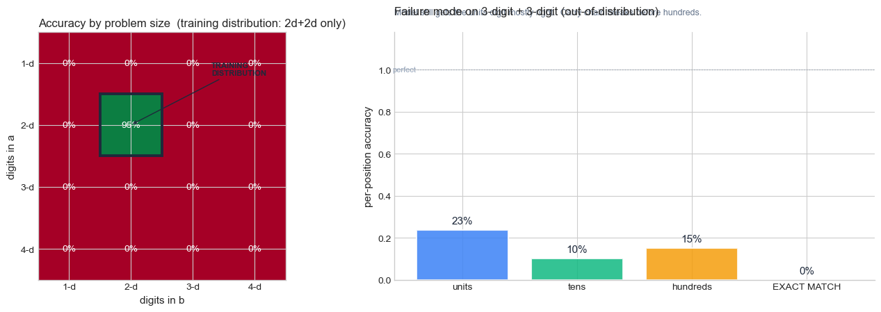
../_images/423e4cde3f148ab1866c5f368ec439ae3f4b09b0c70d32d6b8ea8d34cc96e7f5.png

How to read the figure above. The two panels say complementary things.

Left panel (heatmap). Each cell is the model’s accuracy on a problem class defined by (digits in a, digits in b). The framed cell at (2-d, 2-d) is the only one the model was trained on. Read the row for 2-d a + k-d b: as \(k\) grows, the model breaks even though only one operand changed length. So the failure is not about input complexity in some abstract sense — it is about whether the input distribution matches training.
Right panel (per-position bars). When the model gets a 3+3 problem wrong, which digit of the answer is wrong? The units bar is tall (the model usually gets the rightmost digit right), the tens bar is shorter, and the hundreds bar is the shortest. The exact-match bar is shorter still because a single wrong digit anywhere kills it.

Put the two together: the model has not learned addition as an algorithm (which would generalise), it has learned addition as a table (which does not). The fragment of the algorithm it did pick up — “for the rightmost digit, just add and mod 10” — works because that step has the same form regardless of operand length. Carry propagation does not, because it requires re-applying the same logic an arbitrary number of times. We will return to this distinction (lookup vs algorithm) every time we evaluate generalisation in the rest of the course.

What this teaches us#

Two striking patterns:

The model masters its training distribution (the 2-d + 2-d cell, in dark green) but falls off a cliff the moment we step outside it. This is distribution shift writ tiny.
Inside the failure, the model still gets the units digit mostly right. It gradually loses accuracy on tens, then hundreds — the carry chain breaks before the most significant digit. The model has learned a partial algorithm: copy the rightmost addition correctly but cannot propagate carry further.

The deep lesson: the model has not learned addition; it has compressed a 100×100 lookup table into ~50K parameters. When we ask for a problem outside that table, no algorithm exists in the network to fall back on.

This is compositional generalisation failure. Solving it is one of the deepest open problems in sequence modelling, traceable through:

B. Lake and M. Baroni, “Generalization without Systematicity: On the Compositional Skills of Sequence-to-Sequence Recurrent Networks”, ICML 2018 (arXiv:1711.00350) — the SCAN benchmark, showing seq2seq fails on simple compositional translation.
D. Hupkes et al., “Compositionality Decomposed: How do Neural Networks Generalise?”, JAIR 2020 (arXiv:1908.08351) — a taxonomy of compositional skills.
R. Nogueira, Z. Jiang, J. Lin, “Investigating the Limitations of Transformers with Simple Arithmetic Tasks”, arXiv:2102.13019, 2021 — even Transformers struggle with multi-digit addition.
J. Wei et al., “Chain-of-Thought Prompting Elicits Reasoning in Large Language Models”, NeurIPS 2022 (arXiv:2201.11903) — the modern workaround: prompt the model to write out intermediate steps, turning a one-shot answer into a multi-step computation it can actually do.

Attention (Chapter 37) helps — by letting the decoder look at the digits it is adding, rather than reading them through a single bottleneck. The Transformer (Chapter 40) helps further with explicit positional encoding. But even GPT-4 makes arithmetic errors on long numbers, and the most reliable fix today is to give the model a calculator (tool use). The architectural debate is far from over.

Why arithmetic is the right second example

Reversal demonstrates the bottleneck quantitatively: how much information fits in a fixed vector. Arithmetic demonstrates the bottleneck qualitatively: the kind of computation a fixed-capacity vector can and cannot represent. The model can store enough bits for 10,000 cases but cannot encode the algorithm that would handle the 10,001st. This is the gap between memorisation and understanding.

36.6 The Road Ahead#

The encoder-decoder architecture completes the trajectory of recurrent neural networks that we have traced across Part IX and Part X. Let us place seq2seq in the full historical context:

Show code cell source Hide code cell source

fig, ax = plt.subplots(figsize=(14, 5.5))

events = [
    (1982, 'Hopfield\nNetworks', '#64748b', 'above'),
    (1986, 'Jordan\nNetworks', '#64748b', 'below'),
    (1990, 'Elman\nNetworks (SRN)', '#3b82f6', 'above'),
    (1991, 'Hochreiter:\nVanishing\nGradient', '#dc2626', 'below'),
    (1997, 'LSTM\n(Hochreiter &\nSchmidhuber)', '#059669', 'above'),
    (2000, 'Forget\nGates\n(Gers et al.)', '#059669', 'below'),
    (2014.0, 'GRU\n(Cho et al.)', '#7c3aed', 'above'),
    (2014.3, 'Seq2Seq\n(Sutskever\net al.)', '#f59e0b', 'below'),
    (2014.6, 'Attention\n(Bahdanau\net al.)', '#f59e0b', 'above'),
    (2017, 'Transformer\n(Vaswani\net al.)', '#dc2626', 'below'),
    (2018, 'BERT / GPT\n(Devlin /\nRadford)', '#dc2626', 'above'),
]

# Timeline line
ax.plot([1980, 2020], [0, 0], color='#94a3b8', linewidth=3, zorder=1)

for year, label, color, pos in events:
    side = 1 if pos == 'above' else -1
    y_text = side * 1.6
    y_line = side * 0.5
    
    # Dot
    ax.scatter(year, 0, s=100, color=color, zorder=3, edgecolors='white', linewidth=1.5)
    # Connector
    ax.plot([year, year], [0, y_line], color=color, linewidth=1.5, zorder=2)
    # Label
    ax.text(year, y_text, f'{int(year)}\n{label}', ha='center',
            va='bottom' if side > 0 else 'top',
            fontsize=8, fontweight='bold', color=color,
            bbox=dict(boxstyle='round,pad=0.3', facecolor='white',
                      edgecolor=color, alpha=0.9))

# Highlight regions
ax.axvspan(1982, 2000.5, alpha=0.04, color='#3b82f6')
ax.text(1991, -2.8, 'Part IX: Foundations', ha='center', fontsize=9,
        fontstyle='italic', color='#3b82f6')

ax.axvspan(2000.5, 2015, alpha=0.04, color='#059669')
ax.text(2007.5, -2.8, 'Part X: Sequence\nModeling', ha='center', fontsize=9,
        fontstyle='italic', color='#059669')

ax.axvspan(2015, 2020, alpha=0.04, color='#dc2626')
ax.text(2017.5, -2.8, 'Part XI:\nAttention', ha='center', fontsize=9,
        fontstyle='italic', color='#dc2626')

ax.set_xlim(1979, 2021)
ax.set_ylim(-3.5, 3.8)
ax.set_xlabel('Year', fontsize=11)
ax.set_title('The Road from Recurrence to Attention',
             fontsize=14, fontweight='bold', pad=15)
ax.set_yticks([])
ax.spines['left'].set_visible(False)
ax.spines['right'].set_visible(False)
ax.spines['top'].set_visible(False)

plt.tight_layout()
plt.show()

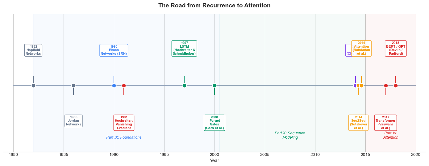
../_images/345b101735e0c5525c335cd7966979b13f578e552092fed7a668596429e6485a.png

The historical arc reveals a consistent pattern: each innovation in recurrent networks addressed a specific limitation of its predecessor.

Problem	Solution	Year
Simple recurrence cannot store long-term dependencies	LSTM gated memory	1997
LSTM cannot learn to forget outdated information	Forget gate	2000
LSTM has many parameters	GRU (simpler gating)	2014
Variable-length input/output	Encoder-decoder (seq2seq)	2014
Fixed-size bottleneck in seq2seq	Attention mechanism	2014
Recurrence is sequential (slow to train)	Transformer (attention only)	2017

The Legacy of RNNs

Transformers have largely replaced RNNs in practice, but the conceptual foundations laid by recurrent networks remain essential:

Sequential processing and the idea that hidden states carry information across time.
Gating mechanisms (forget, update, reset) that control information flow.
Encoder-decoder decomposition of sequence transduction tasks.
Teacher forcing as a training strategy for autoregressive models.

Every one of these ideas, born in the RNN era, lives on in the Transformer architecture and the large language models built upon it. Understanding RNNs is not merely historical—it is the prerequisite for understanding why and how the Transformer works.

Exercises#

Exercise 36.1: Encoder Hidden States#

Consider a unidirectional LSTM encoder with hidden size \(d = 128\) processing a sentence of length \(T = 50\).

(a.) What is the shape of the context vector \(c\)? How many scalar values does it contain?

(b.) How many hidden states \(h_1^{\text{enc}}, \ldots, h_T^{\text{enc}}\) does the encoder produce in total? What are their shapes?

(c.) In the standard seq2seq model, only \(h_T^{\text{enc}}\) is passed to the decoder. What fraction of the encoder’s intermediate computations is directly used?

(d.) The attention mechanism uses all encoder hidden states. If we store them in a matrix, what is its shape? How does this compare to the context vector?

Exercise 36.2: Teacher Forcing Trade-offs#

During training, the decoder can receive either the ground-truth token \(y_{t-1}\) (teacher forcing) or its own prediction \(\hat{y}_{t-1}\) (free running).

(a.) Explain why teacher forcing accelerates training. What distribution does the decoder see during training with teacher forcing?

(b.) At inference time, the model must use its own predictions. This creates a mismatch between training and inference called exposure bias. Describe how errors can compound during free-running generation.

(c.) Suggest a training strategy that interpolates between teacher forcing and free running. (Hint: the teacher_forcing_ratio parameter in our code does exactly this.)

Exercise 36.3: Bidirectional Representations#

A bidirectional LSTM with hidden size \(d\) produces forward states \(\overrightarrow{h}_t \in \mathbb{R}^d\) and backward states \(\overleftarrow{h}_t \in \mathbb{R}^d\).

(a.) What information does \(\overrightarrow{h}_t\) capture that \(\overleftarrow{h}_t\) does not, and vice versa?

(b.) For the string reversal task specifically, explain why a bidirectional encoder has an advantage over a unidirectional one. Which direction’s final state is most useful for the decoder’s first output?

(c.) Why is it inappropriate to use a bidirectional RNN as a decoder in an autoregressive model?

Exercise 36.4: Scaling Laws for the Bottleneck#

Suppose you want to build a seq2seq model that can accurately reverse strings of length up to \(T = 100\).

(a.) For the standard (no-attention) architecture, estimate the minimum hidden size \(d\) needed. Consider that the model must encode 100 characters from a 26-letter alphabet.

(b.) With an attention mechanism, does the hidden size need to scale with the input length? Explain why or why not.

(c.) The Transformer processes all positions in parallel. How does this differ from the sequential processing of RNNs, and what computational advantage does it provide?

Exercise 36.5: Compositional Generalisation in Arithmetic#

In Section 36.5 we trained a seq2seq model on 2-digit + 2-digit addition and observed it fails on 3-digit + 3-digit problems.

(a.) Why does the model still get the units digit right in most failure cases? Reason about which part of the input the decoder’s first output step has the most direct access to.

(b.) Suppose you re-train the same model on a mixture of 2-digit, 3-digit, and 4-digit problems. Predict the result on 5-digit problems. Will the model now generalise? Justify your prediction by analogy with what we observed for 3-digit on a 2-digit-trained model.

(c.) Read the introduction of Lake & Baroni (2018) and explain in 2-3 sentences why string reversal is not a compositional task in their sense, but addition is.

(d.) (Open-ended.) Modern LLMs solve arithmetic via chain-of-thought prompting (Wei et al. 2022): they write out intermediate carry computations as text. Sketch how you would change our seq2seq model so the output is a sequence of intermediate steps (e.g. "7+9=16, carry 1; 4+8+1=13, carry 1; ...") instead of just the final answer. Why might this be easier for a fixed-capacity model to learn?

Summary and Key Takeaways#

The encoder-decoder (seq2seq) architecture maps variable-length input sequences to variable-length output sequences by compressing the input into a fixed-size context vector \(c = h_T^{\text{enc}}\).
Teacher forcing feeds ground-truth tokens to the decoder during training, stabilizing learning but creating exposure bias at inference time.
The bottleneck problem: a single context vector cannot faithfully represent arbitrarily long inputs, causing accuracy to degrade with sequence length.
Bidirectional RNNs give each position access to both left and right context, improving the quality of encoder representations.
The bottleneck motivated attention (Bahdanau et al., 2014), which lets the decoder look at all encoder states, and ultimately led to the Transformer (Vaswani et al., 2017)—the subject of Part XI.

References#

I. Sutskever, O. Vinyals, and Q. V. Le, “Sequence to Sequence Learning with Neural Networks,” Advances in Neural Information Processing Systems (NeurIPS), pp. 3104–3112, 2014.
K. Cho, B. van Merrienboer, C. Gulcehre, D. Bahdanau, F. Bougares, H. Schwenk, and Y. Bengio, “Learning Phrase Representations using RNN Encoder-Decoder for Statistical Machine Translation,” Proceedings of EMNLP, pp. 1724–1734, 2014.
D. Bahdanau, K. Cho, and Y. Bengio, “Neural Machine Translation by Jointly Learning to Align and Translate,” Proceedings of ICLR, 2015. (arXiv preprint 2014.)
M. Schuster and K. K. Paliwal, “Bidirectional Recurrent Neural Networks,” IEEE Transactions on Signal Processing, vol. 45, no. 11, pp. 2673–2681, 1997.
A. Vaswani, N. Shazeer, N. Parmar, J. Uszkoreit, L. Jones, A. N. Gomez, L. Kaiser, and I. Polosukhin, “Attention Is All You Need,” Advances in Neural Information Processing Systems (NeurIPS), pp. 5998–6008, 2017.

Chapter 36: Sequence-to-Sequence and Beyond

Contents

Chapter 36: Sequence-to-Sequence and Beyond#

36.1 The Encoder-Decoder Architecture#

The Encoder#

The Decoder#

A worked example with actual numbers#

36.2 A Toy Seq2Seq: String Reversal#

Building the Model#

Data Generation and Training#

Testing on Short and Long Strings#

36.3 The Bottleneck Problem#

Information-Theoretic Perspective#

How tight is the bottleneck, in numbers?#

36.4 Bidirectional RNNs#

Architecture#

Comparison: Unidirectional vs. Bidirectional Encoder#

36.5 A Harder Task: Arithmetic and the Limits of Memorisation#

Did it learn addition?#

What this teaches us#

36.6 The Road Ahead#

Exercises#

Exercise 36.1: Encoder Hidden States#

Exercise 36.2: Teacher Forcing Trade-offs#

Exercise 36.3: Bidirectional Representations#

Exercise 36.4: Scaling Laws for the Bottleneck#

Exercise 36.5: Compositional Generalisation in Arithmetic#

Summary and Key Takeaways#

References#