Chapter 19: The Universal Approximation Theorem#
The Universal Approximation Theorem (UAT) is one of the most celebrated results in neural network theory. It establishes that feedforward networks with a single hidden layer can approximate any continuous function to arbitrary accuracy, given sufficient width.
This chapter presents the precise statement, develops the constructive intuition, sketches the functional-analytic proof, and critically examines what the theorem does and does not say.
19.1 Statement of the Theorem#
Theorem (Universal Approximation – Hornik, Stinchcombe, White, 1989)
Let \(\sigma: \mathbb{R} \to \mathbb{R}\) be a non-constant, bounded, and continuous activation function (e.g., the sigmoid). Let \(I_n = [0, 1]^n\) be the unit hypercube in \(\mathbb{R}^n\). Let \(f: I_n \to \mathbb{R}\) be any continuous function.
Then for every \(\varepsilon > 0\), there exist an integer \(N\), real constants \(v_i, b_i \in \mathbb{R}\), and vectors \(\mathbf{w}_i \in \mathbb{R}^n\) for \(i = 1, \ldots, N\), such that:
In other words, the set of functions representable by one-hidden-layer networks is dense in \(C(I_n)\) (the space of continuous functions on \(I_n\)) with respect to the supremum norm.
What This Means#
A single hidden layer is sufficient to represent any continuous function, provided the layer is wide enough. The network
is a weighted sum of \(N\) “bumps” (or shifted, scaled activation functions), and \(N\) can always be chosen large enough to approximate \(f\) to within \(\varepsilon\).
Note
Historical note – Cybenko (1989) first proved the Universal Approximation Theorem for sigmoid activations specifically. Hornik, Stinchcombe & White (1989) proved it independently for a broader class of bounded, non-constant continuous activations. Hornik (1991) further generalized the result, and Leshno et al. (1993) showed that the theorem holds for any non-polynomial activation function – including ReLU, which is neither bounded nor sigmoidal.
19.2 Constructive Intuition#
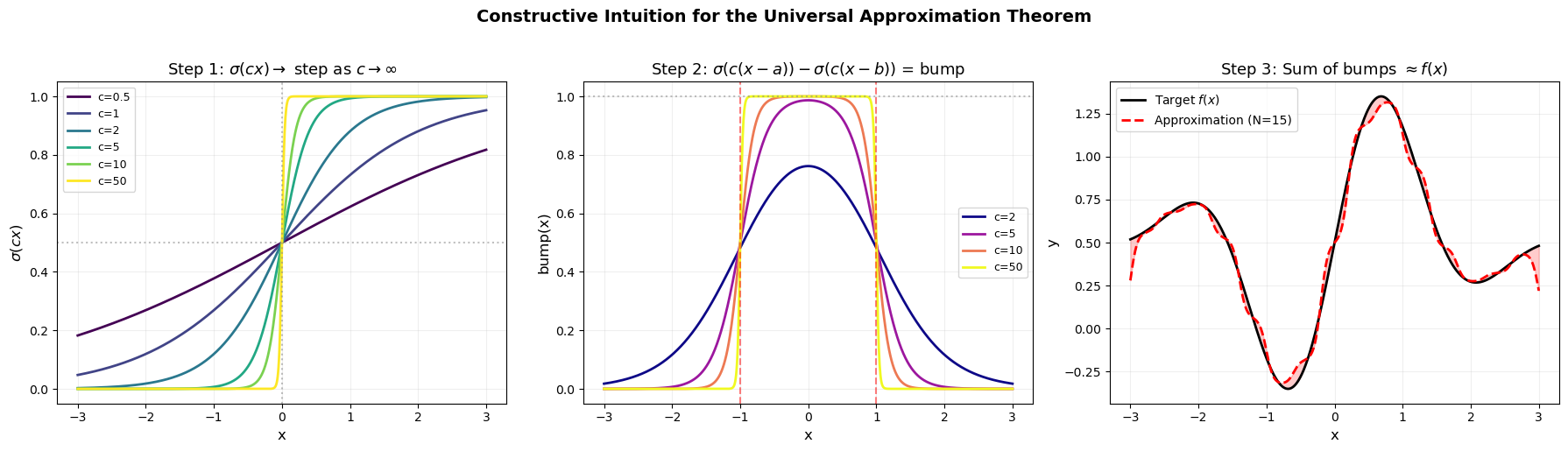
Before the formal proof, let us build geometric intuition for why the theorem is true. The argument proceeds in three steps.
Tip
The bump construction – The key intuition behind the UAT is surprisingly simple. Two sigmoid units can form a “bump” function (nonzero only on a small interval). By stacking many bumps of appropriate heights, we can build a piecewise-constant approximation to ANY continuous function. The finer the bumps, the better the approximation. This constructive argument makes the theorem feel almost obvious once you see it.
Step 1: Sigmoid Becomes a Step Function#
Consider \(\sigma(cx)\) for increasing values of \(c\). As \(c \to \infty\), the sigmoid approaches a step function:
Step 2: Two Steps Make a Bump#
A bump function on the interval \((a, b)\) can be constructed as:
For large \(c\), this is approximately 1 on \((a, b)\) and 0 elsewhere.
Step 3: Bumps Approximate Any Function#
Given a target function \(f\), partition the domain into small intervals and use a scaled bump on each interval:
This is a piecewise constant approximation. As the partition becomes finer (\(N \to \infty\)), \(F \to f\) uniformly.
Show code cell source
import numpy as np
import matplotlib.pyplot as plt

# ============================================================
# Step 1: Sigmoid -> Step Function as c -> infinity
# ============================================================

x = np.linspace(-3, 3, 1000)

fig, axes = plt.subplots(1, 3, figsize=(18, 5))

# Step 1: Sigmoid sharpening
c_values = [0.5, 1, 2, 5, 10, 50]
colors = plt.cm.viridis(np.linspace(0, 1, len(c_values)))

for c, color in zip(c_values, colors):
    axes[0].plot(x, 1/(1+np.exp(-c*x)), color=color, linewidth=2, label=f'c={c}')

axes[0].axhline(y=0.5, color='gray', linestyle=':', alpha=0.5)
axes[0].axvline(x=0, color='gray', linestyle=':', alpha=0.5)
axes[0].set_xlabel('x', fontsize=12)
axes[0].set_ylabel('$\\sigma(cx)$', fontsize=12)
axes[0].set_title('Step 1: $\\sigma(cx) \\to$ step as $c \\to \\infty$', fontsize=13)
axes[0].legend(fontsize=9)
axes[0].grid(True, alpha=0.2)

# Step 2: Two steps make a bump
a, b = -1, 1  # bump on (-1, 1)
c_bump_values = [2, 5, 10, 50]
colors2 = plt.cm.plasma(np.linspace(0, 1, len(c_bump_values)))

for c, color in zip(c_bump_values, colors2):
    bump = 1/(1+np.exp(-c*(x-a))) - 1/(1+np.exp(-c*(x-b)))
    axes[1].plot(x, bump, color=color, linewidth=2, label=f'c={c}')

axes[1].axhline(y=1, color='gray', linestyle=':', alpha=0.5)
axes[1].axvline(x=a, color='red', linestyle='--', alpha=0.5)
axes[1].axvline(x=b, color='red', linestyle='--', alpha=0.5)
axes[1].set_xlabel('x', fontsize=12)
axes[1].set_ylabel('bump(x)', fontsize=12)
axes[1].set_title('Step 2: $\\sigma(c(x-a)) - \\sigma(c(x-b))$ = bump', fontsize=13)
axes[1].legend(fontsize=9)
axes[1].grid(True, alpha=0.2)

# Step 3: Bumps approximate any function
def target_func(x):
    return np.sin(2*x) * np.exp(-0.3*x**2) + 0.5

x_fine = np.linspace(-3, 3, 1000)
axes[2].plot(x_fine, target_func(x_fine), 'k-', linewidth=2, label='Target $f(x)$')

# Approximate with N bumps
N_bumps = 15
c_approx = 20
edges = np.linspace(-3, 3, N_bumps + 1)
centers = (edges[:-1] + edges[1:]) / 2

approx = np.zeros_like(x_fine)
for k in range(N_bumps):
    bump_k = 1/(1+np.exp(-c_approx*(x_fine-edges[k]))) - 1/(1+np.exp(-c_approx*(x_fine-edges[k+1])))
    height = target_func(centers[k])
    approx += height * bump_k

axes[2].plot(x_fine, approx, 'r--', linewidth=2, label=f'Approximation (N={N_bumps})')
axes[2].fill_between(x_fine, target_func(x_fine), approx, alpha=0.2, color='red')
axes[2].set_xlabel('x', fontsize=12)
axes[2].set_ylabel('y', fontsize=12)
axes[2].set_title('Step 3: Sum of bumps $\\approx f(x)$', fontsize=13)
axes[2].legend(fontsize=10)
axes[2].grid(True, alpha=0.2)

plt.suptitle('Constructive Intuition for the Universal Approximation Theorem',
             fontsize=14, fontweight='bold', y=1.02)
plt.tight_layout()
plt.savefig('uat_intuition.png', dpi=150, bbox_inches='tight')
plt.show()
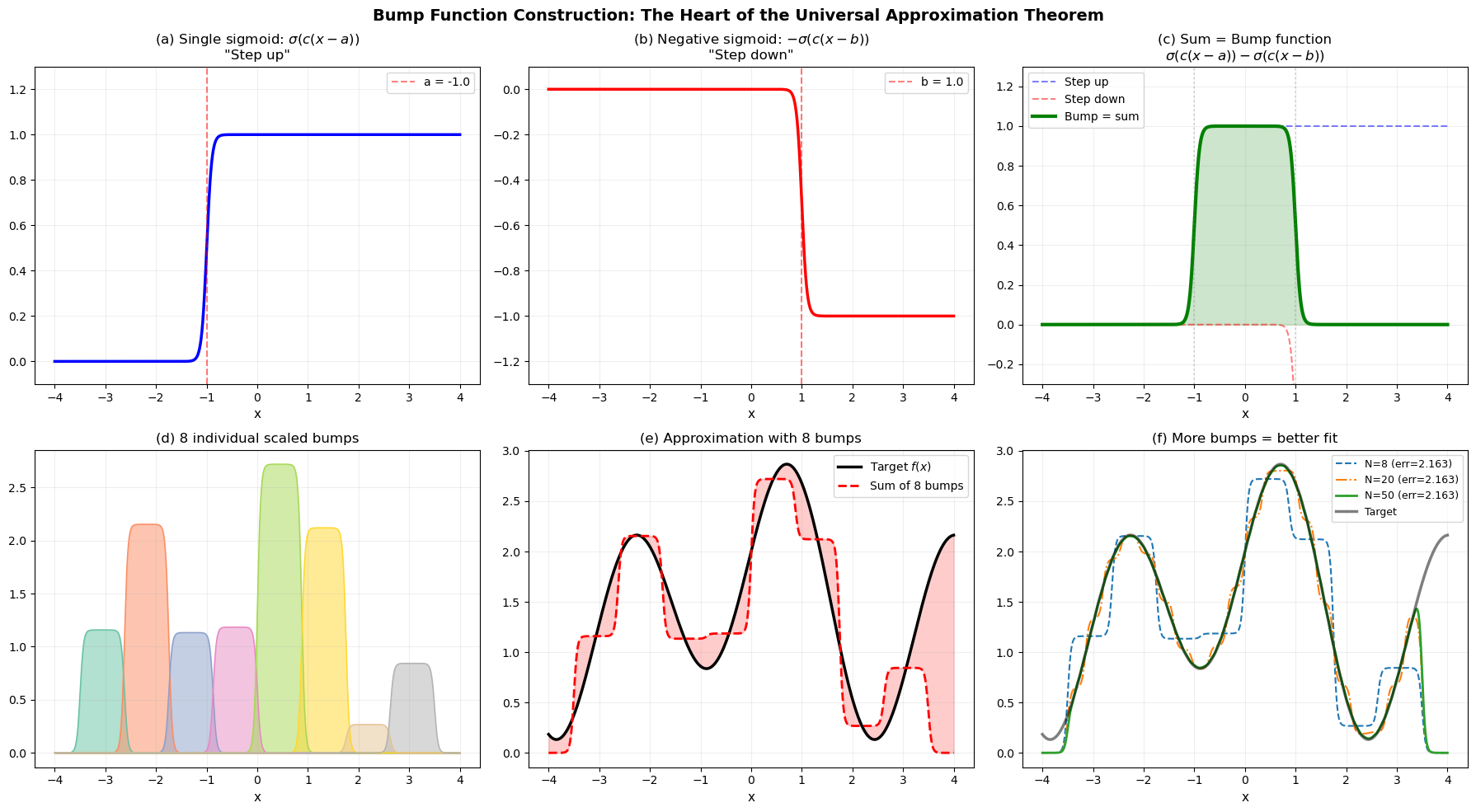
Bump Function Construction – Step by Step#
The following visualization shows the bump construction in detail: how two sigmoid units make a bump, and how many bumps can approximate an arbitrary continuous function.
Show code cell source
import numpy as np
import matplotlib.pyplot as plt

x = np.linspace(-4, 4, 1000)

fig, axes = plt.subplots(2, 3, figsize=(18, 10))

# Panel 1: Single sigmoid (step up)
c = 20
a_pos = -1.0
step_up = 1 / (1 + np.exp(-c * (x - a_pos)))
axes[0, 0].plot(x, step_up, 'b-', linewidth=2.5)
axes[0, 0].axvline(x=a_pos, color='red', linestyle='--', alpha=0.5, label=f'a = {a_pos}')
axes[0, 0].set_title('(a) Single sigmoid: $\\sigma(c(x-a))$\n"Step up"', fontsize=12)
axes[0, 0].set_xlabel('x', fontsize=11)
axes[0, 0].legend(fontsize=10)
axes[0, 0].grid(True, alpha=0.2)
axes[0, 0].set_ylim(-0.1, 1.3)

# Panel 2: Negative sigmoid (step down)
b_pos = 1.0
step_down = -1 / (1 + np.exp(-c * (x - b_pos)))
axes[0, 1].plot(x, step_down, 'r-', linewidth=2.5)
axes[0, 1].axvline(x=b_pos, color='red', linestyle='--', alpha=0.5, label=f'b = {b_pos}')
axes[0, 1].set_title('(b) Negative sigmoid: $-\\sigma(c(x-b))$\n"Step down"', fontsize=12)
axes[0, 1].set_xlabel('x', fontsize=11)
axes[0, 1].legend(fontsize=10)
axes[0, 1].grid(True, alpha=0.2)
axes[0, 1].set_ylim(-1.3, 0.1)

# Panel 3: Sum = bump
bump = step_up + step_down
axes[0, 2].plot(x, step_up, 'b--', linewidth=1.5, alpha=0.5, label='Step up')
axes[0, 2].plot(x, step_down, 'r--', linewidth=1.5, alpha=0.5, label='Step down')
axes[0, 2].plot(x, bump, 'g-', linewidth=3, label='Bump = sum')
axes[0, 2].fill_between(x, 0, bump, alpha=0.2, color='green')
axes[0, 2].axvline(x=a_pos, color='gray', linestyle=':', alpha=0.3)
axes[0, 2].axvline(x=b_pos, color='gray', linestyle=':', alpha=0.3)
axes[0, 2].set_title('(c) Sum = Bump function\n$\\sigma(c(x-a)) - \\sigma(c(x-b))$', fontsize=12)
axes[0, 2].set_xlabel('x', fontsize=11)
axes[0, 2].legend(fontsize=10)
axes[0, 2].grid(True, alpha=0.2)
axes[0, 2].set_ylim(-0.3, 1.3)

# Panel 4: Multiple bumps (individual)
def target_fn(x):
    return np.sin(2*x) + 0.5*np.cos(x) + 1.5

N = 8
edges = np.linspace(-3.5, 3.5, N + 1)
centers = (edges[:-1] + edges[1:]) / 2
c_sharp = 30

bump_colors = plt.cm.Set2(np.linspace(0, 1, N))
for k in range(N):
    bump_k = 1/(1+np.exp(-c_sharp*(x-edges[k]))) - 1/(1+np.exp(-c_sharp*(x-edges[k+1])))
    height_k = target_fn(centers[k])
    axes[1, 0].fill_between(x, 0, height_k * bump_k, alpha=0.5, color=bump_colors[k])
    axes[1, 0].plot(x, height_k * bump_k, color=bump_colors[k], linewidth=1)

axes[1, 0].set_title(f'(d) {N} individual scaled bumps', fontsize=12)
axes[1, 0].set_xlabel('x', fontsize=11)
axes[1, 0].grid(True, alpha=0.2)

# Panel 5: Sum of bumps vs target
approx = np.zeros_like(x)
for k in range(N):
    bump_k = 1/(1+np.exp(-c_sharp*(x-edges[k]))) - 1/(1+np.exp(-c_sharp*(x-edges[k+1])))
    approx += target_fn(centers[k]) * bump_k

axes[1, 1].plot(x, target_fn(x), 'k-', linewidth=2.5, label='Target $f(x)$')
axes[1, 1].plot(x, approx, 'r--', linewidth=2, label=f'Sum of {N} bumps')
axes[1, 1].fill_between(x, target_fn(x), approx, alpha=0.2, color='red')
axes[1, 1].set_title(f'(e) Approximation with {N} bumps', fontsize=12)
axes[1, 1].set_xlabel('x', fontsize=11)
axes[1, 1].legend(fontsize=10)
axes[1, 1].grid(True, alpha=0.2)

# Panel 6: Better approximation with more bumps
for N_fine, lstyle, lw in [(8, '--', 1.5), (20, '-.', 1.5), (50, '-', 2)]:
    edges_f = np.linspace(-3.5, 3.5, N_fine + 1)
    centers_f = (edges_f[:-1] + edges_f[1:]) / 2
    approx_f = np.zeros_like(x)
    for k in range(N_fine):
        bump_k = 1/(1+np.exp(-c_sharp*(x-edges_f[k]))) - 1/(1+np.exp(-c_sharp*(x-edges_f[k+1])))
        approx_f += target_fn(centers_f[k]) * bump_k
    error = np.max(np.abs(target_fn(x) - approx_f))
    axes[1, 2].plot(x, approx_f, linestyle=lstyle, linewidth=lw,
                    label=f'N={N_fine} (err={error:.3f})')

axes[1, 2].plot(x, target_fn(x), 'k-', linewidth=2.5, label='Target', alpha=0.5)
axes[1, 2].set_title('(f) More bumps = better fit', fontsize=12)
axes[1, 2].set_xlabel('x', fontsize=11)
axes[1, 2].legend(fontsize=9)
axes[1, 2].grid(True, alpha=0.2)

plt.suptitle('Bump Function Construction: The Heart of the Universal Approximation Theorem',
             fontsize=14, fontweight='bold')
plt.tight_layout()
plt.savefig('bump_construction.png', dpi=150, bbox_inches='tight')
plt.show()
19.3 Cybenko’s Proof Sketch#
The first rigorous proof was given by Cybenko (1989), using functional analysis. Here we outline the key ideas.
Proof Sketch
Setup. Let \(\Sigma \subset C(I_n)\) be the set of all functions of the form:
Let \(\overline{\Sigma}\) be the closure of \(\Sigma\) in \(C(I_n)\) (w.r.t. supremum norm).
Goal: Show \(\overline{\Sigma} = C(I_n)\).
Step 1 (Hahn-Banach): Assume for contradiction that \(\overline{\Sigma} \neq C(I_n)\). Since \(\overline{\Sigma}\) is a proper closed subspace of \(C(I_n)\), by the Hahn-Banach theorem there exists a nonzero bounded linear functional \(\Lambda \in C(I_n)^*\) such that \(\Lambda(F) = 0\) for all \(F \in \overline{\Sigma}\).
Step 2 (Riesz Representation): By the Riesz representation theorem, there exists a nonzero signed Borel measure \(\mu\) on \(I_n\) such that:
Step 3 (Consequence): Since \(\Lambda\) vanishes on \(\Sigma\), for all \(\mathbf{w} \in \mathbb{R}^n\) and \(b \in \mathbb{R}\):
Step 4 (Key Technical Step): Using the fact that \(\sigma\) is a discriminatory function (a property defined by Cybenko), one can show that the Fourier transform of \(\mu\) vanishes identically. Since the Fourier transform is injective on measures, this implies \(\mu = 0\).
Step 5 (Contradiction): But \(\mu\) was assumed to be nonzero. Contradiction. Therefore \(\overline{\Sigma} = C(I_n)\). \(\blacksquare\)
Key Definition: A function \(\sigma\) is discriminatory if the only signed measure \(\mu\) satisfying \(\int \sigma(\mathbf{w}^\top \mathbf{x} + b) \, d\mu = 0\) for all \(\mathbf{w}, b\) is \(\mu = 0\). Cybenko showed that any bounded, continuous sigmoidal function is discriminatory.
19.4 What the UAT Tells Us vs. What It Does Not#
What the UAT Tells Us#
Existence: For any continuous function and any desired accuracy, there exists a one-hidden-layer network that achieves that accuracy.
Universality: One hidden layer is sufficient (in principle) for any approximation task.
Expressiveness: Neural networks are not inherently limited in what they can represent.
What the UAT Does NOT Tell Us#
Required width \(N\): The theorem gives no bound on how many hidden neurons are needed. For some functions, \(N\) may be astronomically large (exponential in the input dimension).
Learnability: The theorem says good parameters exist, but not that gradient descent (or any algorithm) can find them. Finding the optimal weights is NP-hard in general.
Generalization: Approximating \(f\) on the training set does not guarantee good performance on unseen data. The theorem is purely about representation, not statistical learning.
Depth efficiency: The theorem does not address whether deeper networks can be exponentially more efficient than shallow ones (they can – see Section 19.5).
Sample complexity: How many training samples are needed? The UAT says nothing about this.
Danger
❗ Existence does not equal Learnability! The UAT proves that a solution EXISTS but says NOTHING about how to FIND it. Gradient descent may not converge to the universal approximator. The loss landscape could have bad local minima, saddle points, or plateaus that prevent any practical optimization algorithm from finding the right weights. This is perhaps the most commonly misunderstood theorem in ML.
Danger
❗ The required number of neurons may be EXPONENTIALLY large. For some functions, a single hidden layer needs exponentially many neurons (in the input dimension), while a deep network needs only polynomial. For example, computing the parity of \(n\) binary inputs requires \(2^n\) hidden neurons with one layer, but only \(O(n)\) with \(O(\log n)\) layers. The UAT guarantees a solution exists but it may be impractically wide.
Warning
Depth vs Width tradeoff – The UAT focuses on width (single hidden layer), but modern deep learning shows that depth wins empirically. Depth can be much more parameter-efficient for some function classes, and empirically deep models often work better. The UAT itself, however, does not prove better generalization or superior efficiency for every problem.
19.5 Depth Separation#
While the UAT shows that width is sufficient for universality, depth provides exponential efficiency.
Telgarsky’s Theorem (2016)#
There exist functions computable by a network of depth \(O(k)\) and polynomial width that require exponential width \(2^{\Omega(k)}\) to approximate with a network of depth \(O(1)\) (constant depth).
Intuition#
Deep networks can compose functions:
Each layer applies a nonlinear transformation.
With \(L\) layers, the network computes a composition of \(L\) nonlinear maps.
This allows exponential growth in the number of linear regions.
A ReLU network with \(L\) layers and \(n\) neurons per layer can represent a piecewise linear function with up to \(O\left(\binom{n}{d}^L\right)\) linear regions, where \(d\) is the input dimension. Compare this with \(O(n)\) regions for a single layer.
The Lesson#
Depth is not just a convenience – it is fundamentally more powerful than width. This theoretical result aligns with the practical success of deep networks.
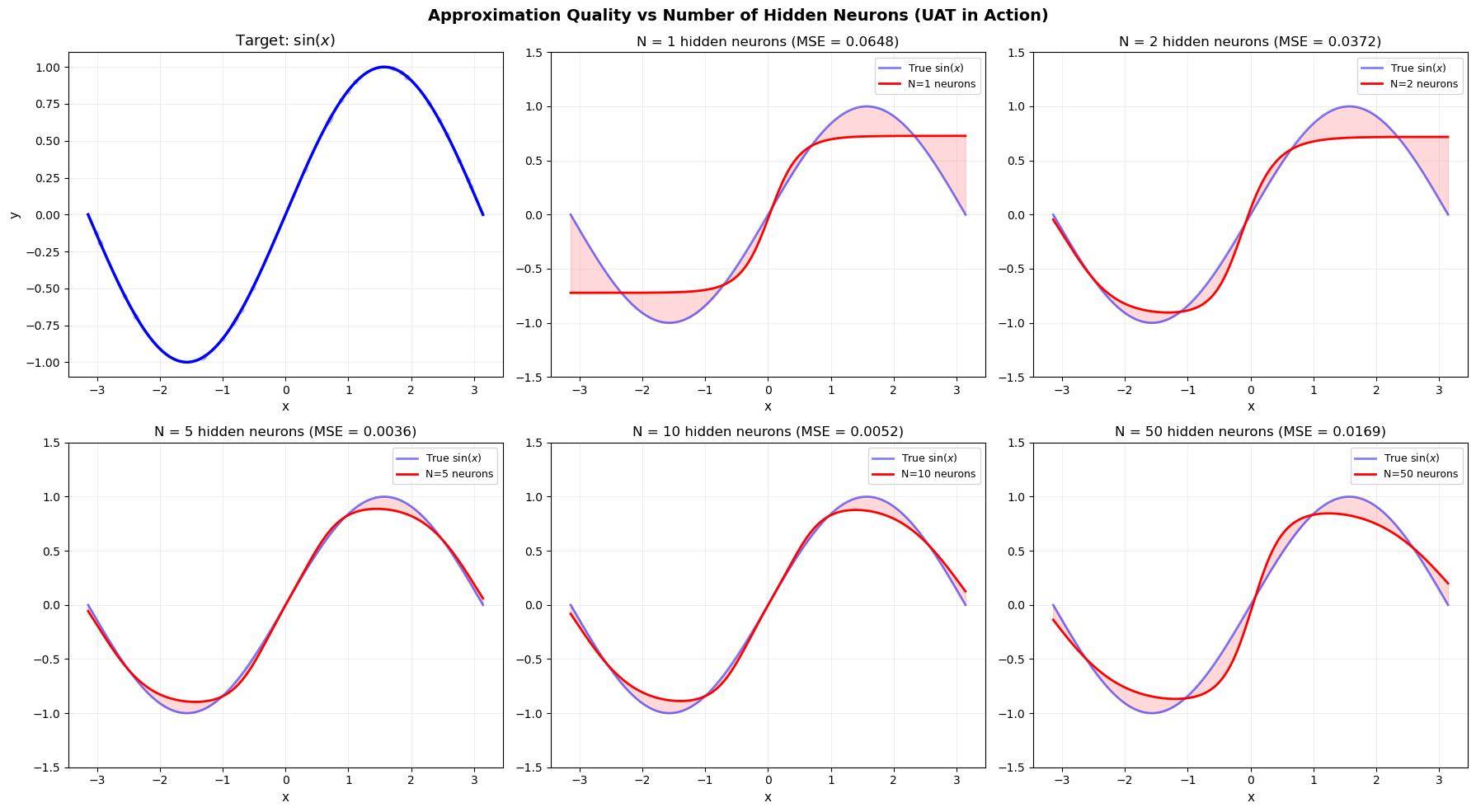
Show code cell source
# Demonstration: Approximation quality improves with N
import numpy as np
import matplotlib.pyplot as plt
def target_function(x):
"""A complex target function to approximate."""
return np.sin(3*x) * np.cos(x) + 0.3 * np.sin(7*x)
def sigmoid(z):
return 1 / (1 + np.exp(-np.clip(z, -500, 500)))
def bump_approximation(x, N, target_fn, x_min=-3, x_max=3, sharpness=30):
"""Approximate target_fn using N bump functions."""
edges = np.linspace(x_min, x_max, N + 1)
centers = (edges[:-1] + edges[1:]) / 2
approx = np.zeros_like(x)
for k in range(N):
bump = sigmoid(sharpness * (x - edges[k])) - sigmoid(sharpness * (x - edges[k+1]))
approx += target_fn(centers[k]) * bump
return approx
x = np.linspace(-3, 3, 1000)
y_true = target_function(x)
N_values = [3, 5, 10, 20, 50]
fig, axes = plt.subplots(2, 3, figsize=(18, 10))
axes = axes.flatten()
# First panel: true function
axes[0].plot(x, y_true, 'b-', linewidth=2)
axes[0].set_title('Target function $f(x)$', fontsize=12)
axes[0].grid(True, alpha=0.2)
for idx, N in enumerate(N_values):
ax = axes[idx + 1]
y_approx = bump_approximation(x, N, target_function)
ax.plot(x, y_true, 'b-', linewidth=2, alpha=0.5, label='True')
ax.plot(x, y_approx, 'r-', linewidth=2, label=f'N={N}')
error = np.max(np.abs(y_true - y_approx))
ax.set_title(f'N = {N} bumps (max error: {error:.3f})', fontsize=12)
ax.legend(fontsize=9)
ax.grid(True, alpha=0.2)
plt.suptitle('Universal Approximation: More neurons $\\Rightarrow$ better approximation',
fontsize=14, fontweight='bold')
plt.tight_layout()
plt.savefig('uat_demonstration.png', dpi=150, bbox_inches='tight')
plt.show()
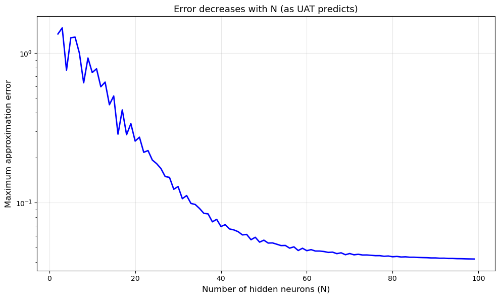
# Error vs N
N_range = range(2, 100)
errors = []
for N in N_range:
y_approx = bump_approximation(x, N, target_function)
errors.append(np.max(np.abs(y_true - y_approx)))
fig, ax = plt.subplots(figsize=(10, 6))
ax.plot(list(N_range), errors, 'b-', linewidth=2)
ax.set_xlabel('Number of hidden neurons (N)', fontsize=12)
ax.set_ylabel('Maximum approximation error', fontsize=12)
ax.set_title('Error decreases with N (as UAT predicts)', fontsize=13)
ax.set_yscale('log')
ax.grid(True, alpha=0.3)
plt.tight_layout()
plt.savefig('uat_error_vs_N.png', dpi=150, bbox_inches='tight')
plt.show()

19.6 Extensions: Leshno et al. (1993)#
The original UAT by Cybenko (1989) and Hornik et al. (1989) required the activation function to be sigmoidal (bounded, continuous, with appropriate limiting behavior).
Theorem (Leshno, Lin, Pinkus & Schocken, 1993):
A standard feedforward network with a single hidden layer can approximate any continuous function on compact subsets of \(\mathbb{R}^n\) if and only if the activation function \(\sigma\) is not a polynomial.
Implications#
ReLU works: \(\text{ReLU}(x) = \max(0, x)\) is not a polynomial, so ReLU networks are universal approximators. This is important because ReLU is not bounded and not sigmoidal.
Polynomials fail: If \(\sigma(x) = x^k\) (a polynomial), then the network can only represent polynomials, which are not dense in \(C(I_n)\).
Nearly any nonlinearity works: The theorem is remarkably general – essentially any nonlinear activation function (other than polynomials) gives universality.
This explains the practical observation that neural networks work with a wide variety of activation functions: sigmoid, tanh, ReLU, ELU, GELU, etc.
Exercises#
Exercise 19.1. Construct a bump function approximation of \(f(x) = e^{-x^2}\) on \([-3, 3]\) using \(N = 5, 10, 20, 50\) sigmoid bumps. Plot the approximation error as a function of \(N\).
Exercise 19.2. Extend the bump construction to 2D. Approximate \(f(x_1, x_2) = \sin(x_1) \cos(x_2)\) on \([-\pi, \pi]^2\) using a grid of 2D bump functions. Visualize the true function and the approximation as surface plots.
Exercise 19.3. Train a 1-hidden-layer network (with varying widths \(N = 4, 16, 64, 256\)) to approximate \(f(x) = |x|\) on \([-1, 1]\). Compare the trained approximation quality with the constructive bump approximation.
Exercise 19.4. Demonstrate depth separation empirically. Compare a network with 1 hidden layer of 1000 neurons vs. a network with 5 hidden layers of 10 neurons each (both with ~1000 parameters) on a target function of your choice. Which approximates better?
Exercise 19.5. Why does the UAT not guarantee that gradient descent can find the approximating network? Give a concrete example of a function where the UAT guarantees existence of a good network, but gradient descent from random initialization frequently fails.