Chapter 26: Cross-Entropy, KL Divergence, and Maximum Likelihood#
In 1948, Claude Shannon published A Mathematical Theory of Communication while working at Bell Laboratories, founding the field of information theory and providing a rigorous mathematical framework for quantifying uncertainty. Shannon’s entropy, inspired by the thermodynamic entropy of Boltzmann and Gibbs, gave us a precise measure of the “surprise” or “information content” in a random variable. Three years later, Solomon Kullback and Richard Leibler introduced their divergence measure in On Information and Sufficiency (1951), providing a way to quantify how one probability distribution differs from another. These information-theoretic tools, developed for communication engineering and statistics, would become the foundation of modern loss functions in neural networks.
The connection to learning was made explicit through maximum likelihood estimation, an idea with roots in the work of Daniel Bernoulli (1778) and Carl Friedrich Gauss, later formalized by Ronald Fisher in his landmark 1922 paper. When Rumelhart, Hinton, and Williams popularized backpropagation in 1986, they recognized that the cross-entropy loss—equivalent to the negative log-likelihood—provided superior training dynamics compared to mean squared error for classification tasks. The insight was profound: minimizing cross-entropy is the same as minimizing the KL divergence between the data distribution and the model, which is the same as performing maximum likelihood estimation. This chapter traces these deep connections.
Show code cell source
import numpy as np
import matplotlib.pyplot as plt

plt.style.use('seaborn-v0_8-whitegrid')

# Color palette
BLUE = '#3b82f6'
DARK_BLUE = '#2563eb'
GREEN = '#059669'
AMBER = '#d97706'
RED = '#dc2626'
BURGUNDY = '#8c2f39'
CREAM = '#fdf6e3'

rng = np.random.default_rng(42)
print('Imports loaded. NumPy version:', np.__version__)
Imports loaded. NumPy version: 1.26.4
26.1 Information and Entropy#
Shannon’s Surprise#
Shannon began with a simple question: how much “information” does an event carry? If an event with probability \(p\) occurs, the self-information (or surprisal) is:
This satisfies natural axioms: certain events (\(p = 1\)) carry zero information, rare events (\(p \approx 0\)) carry a lot, and the information from independent events is additive.
Shannon Entropy#
The entropy of a discrete probability distribution \(p = (p_1, p_2, \ldots, p_n)\) is the expected surprisal:
where we adopt the convention \(0 \log 0 = 0\) (justified by continuity). Unless otherwise stated, we use natural logarithm \(\ln\) throughout this chapter (the choice of base only changes the unit of measurement).
Shannon showed that \(H(p)\) represents:
The average surprise when drawing from \(p\),
The minimum average number of bits needed to encode outcomes from \(p\),
A measure of the uncertainty or disorder in the distribution.
Theorem 26.1 (Maximum Entropy)
Among all discrete probability distributions on \(n\) outcomes, the uniform distribution \(p_i = 1/n\) uniquely maximizes the entropy, achieving \(H(p) = \ln n\).
Proof
We maximize \(H(p) = -\sum_{i=1}^{n} p_i \ln p_i\) subject to the constraint \(\sum_{i=1}^{n} p_i = 1\).
Using a Lagrange multiplier \(\lambda\), we form the Lagrangian:
Taking partial derivatives and setting them to zero:
Since the right-hand side is the same for every \(i\), all \(p_i\) are equal. The constraint \(\sum p_i = 1\) gives \(p_i = 1/n\) for all \(i\).
Substituting back:
To confirm this is a maximum (not a minimum), note that \(H\) is a strictly concave function of \(p\) (since \(-p \ln p\) is strictly concave), so any critical point of the Lagrangian on the simplex is a global maximum. \(\blacksquare\)
def entropy(p):
    """Compute Shannon entropy H(p) in nats.

    Parameters
    ----------
    p : array-like
        Probability distribution (must sum to 1, entries >= 0).

    Returns
    -------
    float
        Shannon entropy in nats (natural log units).
    """
    p = np.asarray(p, dtype=float)
    # Filter out zero entries to avoid log(0)
    mask = p > 0
    return -np.sum(p[mask] * np.log(p[mask]))


# Compute entropy for several distributions over 4 outcomes
distributions = {
    'Uniform [0.25, 0.25, 0.25, 0.25]': [0.25, 0.25, 0.25, 0.25],
    'Peaked  [0.70, 0.10, 0.10, 0.10]': [0.70, 0.10, 0.10, 0.10],
    'Skewed  [0.97, 0.01, 0.01, 0.01]': [0.97, 0.01, 0.01, 0.01],
    'Certain [1.00, 0.00, 0.00, 0.00]': [1.00, 0.00, 0.00, 0.00],
}

print(f'{"Distribution":<42s} {"H(p) (nats)":>12s} {"H(p) (bits)":>12s}')
print('-' * 68)
for name, p in distributions.items():
    h = entropy(p)
    print(f'{name:<42s} {h:>12.4f} {h / np.log(2):>12.4f}')

print(f'\nTheoretical max entropy for n=4: ln(4) = {np.log(4):.4f} nats')
Distribution                                H(p) (nats)  H(p) (bits)
--------------------------------------------------------------------
Uniform [0.25, 0.25, 0.25, 0.25]                 1.3863       2.0000
Peaked  [0.70, 0.10, 0.10, 0.10]                 0.9404       1.3568
Skewed  [0.97, 0.01, 0.01, 0.01]                 0.1677       0.2419
Certain [1.00, 0.00, 0.00, 0.00]                -0.0000      -0.0000

Theoretical max entropy for n=4: ln(4) = 1.3863 nats
Show code cell source
# Binary entropy function: H(p) = -p*log(p) - (1-p)*log(1-p)
fig, axes = plt.subplots(1, 2, figsize=(12, 4.5))
fig.patch.set_facecolor(CREAM)
for ax in axes:
    ax.set_facecolor(CREAM)

# Left: binary entropy
p_vals = np.linspace(0.001, 0.999, 500)
h_binary = -p_vals * np.log(p_vals) - (1 - p_vals) * np.log(1 - p_vals)

axes[0].plot(p_vals, h_binary, color=DARK_BLUE, linewidth=2.5)
axes[0].axhline(y=np.log(2), color=AMBER, linestyle='--', alpha=0.7, label=r'$\ln 2$ (maximum)')
axes[0].axvline(x=0.5, color=AMBER, linestyle='--', alpha=0.7)
axes[0].set_xlabel('Probability $p$', fontsize=12)
axes[0].set_ylabel('$H(p)$ (nats)', fontsize=12)
axes[0].set_title('Binary Entropy Function', fontsize=13, fontweight='bold')
axes[0].legend(fontsize=11)
axes[0].set_xlim(0, 1)
axes[0].set_ylim(0, 0.8)

# Right: entropy vs n for uniform distributions
n_values = np.arange(2, 21)
h_uniform = np.log(n_values)

axes[1].bar(n_values, h_uniform, color=BLUE, alpha=0.8, edgecolor='white')
axes[1].set_xlabel('Number of outcomes $n$', fontsize=12)
axes[1].set_ylabel(r'$H_{\max} = \ln n$ (nats)', fontsize=12)
axes[1].set_title('Maximum Entropy vs. Number of Outcomes', fontsize=13, fontweight='bold')
axes[1].set_xticks(n_values[::2])

plt.tight_layout()
plt.show()

The binary entropy curve reveals the key intuition: entropy is maximized when the outcome is most uncertain (\(p = 0.5\)) and minimized when the outcome is deterministic (\(p = 0\) or \(p = 1\)). Shannon proved that entropy is the unique function satisfying continuity, monotonicity for uniform distributions, and the chain rule for compound events.
26.2 Cross-Entropy and KL Divergence#
Cross-Entropy#
Suppose the true distribution of outcomes is \(p\), but we design a coding scheme optimized for a different distribution \(q\). The cross-entropy measures the average number of nats needed:
Since we are using a suboptimal code, we always have \(H(p, q) \geq H(p)\)—we can never do better than the code matched to the true distribution.
Kullback-Leibler Divergence#
The excess cost of using \(q\) instead of \(p\) is the Kullback-Leibler divergence (also called relative entropy):
Kullback and Leibler (1951) introduced this quantity in the context of statistical hypothesis testing, showing it measures the expected log-likelihood ratio between \(p\) and \(q\).
Theorem 26.2 (Gibbs’ Inequality)
\(D_{\text{KL}}(p \,\|\, q) \geq 0\) for all distributions \(p, q\), with equality if and only if \(p = q\).
Proof
We use Jensen’s inequality: for a convex function \(f\) and random variable \(X\), \(f(\mathbb{E}[X]) \leq \mathbb{E}[f(X)].\)
Since \(-\log\) is strictly convex, we have:
Applying Jensen’s inequality with \(f(x) = -\log(x)\) (convex) to the random variable \(X = q_i / p_i\) with probabilities \(p_i\):
Therefore \(-D_{\text{KL}}(p \,\|\, q) \leq 0\), i.e., \(D_{\text{KL}}(p \,\|\, q) \geq 0\).
Equality holds if and only if \(q_i / p_i\) is constant for all \(i\) (strict convexity of \(-\log\)), which combined with \(\sum p_i = \sum q_i = 1\) forces \(p = q\). \(\blacksquare\)
Theorem 26.3 (Minimizing Cross-Entropy Equals Minimizing KL Divergence)
For a fixed true distribution \(p\), minimizing the cross-entropy \(H(p, q)\) over \(q\) is equivalent to minimizing \(D_{\text{KL}}(p \,\|\, q)\) over \(q\).
Proof
Since \(D_{\text{KL}}(p \,\|\, q) = H(p, q) - H(p)\) and \(H(p)\) depends only on \(p\) (not on \(q\)), we have:
This is a simple but crucial observation: when training a model \(q\) to match data distributed as \(p\), minimizing cross-entropy and minimizing KL divergence are the same optimization problem. \(\blacksquare\)
The Asymmetry of KL Divergence
KL divergence is not symmetric: \(D_{\text{KL}}(p \,\|\, q) \neq D_{\text{KL}}(q \,\|\, p)\) in general. It is therefore not a true distance metric. The two directions have different practical meanings:
Forward KL \(D_{\text{KL}}(p \,\|\, q)\): penalizes \(q\) for placing low probability where \(p\) has high probability. Tends to produce mean-seeking (covering) approximations.
Reverse KL \(D_{\text{KL}}(q \,\|\, p)\): penalizes \(q\) for placing high probability where \(p\) has low probability. Tends to produce mode-seeking (concentrated) approximations.
def kl_divergence(p, q):
    """Compute KL divergence D_KL(p || q) in nats.

    Parameters
    ----------
    p, q : array-like
        Probability distributions (must sum to 1).

    Returns
    -------
    float
        KL divergence. Returns inf if q_i = 0 where p_i > 0.
    """
    p = np.asarray(p, dtype=float)
    q = np.asarray(q, dtype=float)
    # Where p > 0, q must be > 0; otherwise KL is infinite
    mask = p > 0
    if np.any(q[mask] <= 0):
        return np.inf
    return np.sum(p[mask] * np.log(p[mask] / q[mask]))


def cross_entropy(p, q):
    """Compute cross-entropy H(p, q) in nats."""
    p = np.asarray(p, dtype=float)
    q = np.asarray(q, dtype=float)
    mask = p > 0
    if np.any(q[mask] <= 0):
        return np.inf
    return -np.sum(p[mask] * np.log(q[mask]))


# Demonstrate the relationship H(p,q) = H(p) + D_KL(p||q)
p = np.array([0.4, 0.3, 0.2, 0.1])
q = np.array([0.1, 0.2, 0.3, 0.4])

h_p = entropy(p)
h_pq = cross_entropy(p, q)
d_kl = kl_divergence(p, q)

print('Demonstrating: H(p, q) = H(p) + D_KL(p || q)')
print(f'  p = {p}')
print(f'  q = {q}')
print(f'  H(p)          = {h_p:.6f}')
print(f'  H(p, q)       = {h_pq:.6f}')
print(f'  D_KL(p || q)  = {d_kl:.6f}')
print(f'  H(p) + D_KL   = {h_p + d_kl:.6f}  (should equal H(p,q))')
print()

# Demonstrate asymmetry
d_kl_forward = kl_divergence(p, q)
d_kl_reverse = kl_divergence(q, p)
print('Demonstrating asymmetry: D_KL(p||q) != D_KL(q||p)')
print(f'  D_KL(p || q) = {d_kl_forward:.6f}')
print(f'  D_KL(q || p) = {d_kl_reverse:.6f}')
print(f'  Difference   = {abs(d_kl_forward - d_kl_reverse):.6f}')
Demonstrating: H(p, q) = H(p) + D_KL(p || q)
  p = [0.4 0.3 0.2 0.1]
  q = [0.1 0.2 0.3 0.4]
  H(p)          = 1.279854
  H(p, q)       = 1.736289
  D_KL(p || q)  = 0.456435
  H(p) + D_KL   = 1.736289  (should equal H(p,q))

Demonstrating asymmetry: D_KL(p||q) != D_KL(q||p)
  D_KL(p || q) = 0.456435
  D_KL(q || p) = 0.456435
  Difference   = 0.000000
Show code cell source
# Visualize KL divergence asymmetry for binary distributions
fig, axes = plt.subplots(1, 2, figsize=(12, 4.5))
fig.patch.set_facecolor(CREAM)
for ax in axes:
    ax.set_facecolor(CREAM)

p_fixed = 0.3
q_range = np.linspace(0.01, 0.99, 300)

# D_KL(p || q) as a function of q, for fixed p
kl_forward = np.array([
    kl_divergence([p_fixed, 1 - p_fixed], [q_val, 1 - q_val])
    for q_val in q_range
])

# D_KL(q || p) as a function of q, for fixed p
kl_reverse = np.array([
    kl_divergence([q_val, 1 - q_val], [p_fixed, 1 - p_fixed])
    for q_val in q_range
])

# Left: both directions on same plot
axes[0].plot(q_range, kl_forward, color=DARK_BLUE, linewidth=2.5,
             label=r'$D_{KL}(p\,\|\,q)$ (forward)')
axes[0].plot(q_range, kl_reverse, color=RED, linewidth=2.5, linestyle='--',
             label=r'$D_{KL}(q\,\|\,p)$ (reverse)')
axes[0].axvline(x=p_fixed, color=GREEN, linestyle=':', linewidth=2,
                label=f'$p = {p_fixed}$')
axes[0].set_xlabel('$q$', fontsize=12)
axes[0].set_ylabel('KL Divergence (nats)', fontsize=12)
axes[0].set_title(f'KL Divergence Asymmetry (fixed $p = {p_fixed}$)',
                   fontsize=13, fontweight='bold')
axes[0].legend(fontsize=10)
axes[0].set_ylim(0, 4)

# Right: heatmap of D_KL(p||q) for binary case
p_grid = np.linspace(0.01, 0.99, 100)
q_grid = np.linspace(0.01, 0.99, 100)
P, Q = np.meshgrid(p_grid, q_grid)
KL = np.zeros_like(P)
for i in range(len(p_grid)):
    for j in range(len(q_grid)):
        KL[j, i] = kl_divergence([P[j, i], 1 - P[j, i]],
                                  [Q[j, i], 1 - Q[j, i]])

KL_clipped = np.clip(KL, 0, 3)
im = axes[1].contourf(P, Q, KL_clipped, levels=20, cmap='Blues')
axes[1].plot([0, 1], [0, 1], color=RED, linestyle='--', linewidth=2,
             label='$p = q$ (zero divergence)')
axes[1].set_xlabel('$p$', fontsize=12)
axes[1].set_ylabel('$q$', fontsize=12)
axes[1].set_title(r'$D_{KL}(p\,\|\,q)$ for Binary Distributions',
                   fontsize=13, fontweight='bold')
axes[1].legend(fontsize=10, loc='upper left')
plt.colorbar(im, ax=axes[1], label='nats')

fig.subplots_adjust(left=0.06, right=0.95, wspace=0.35)
plt.show()
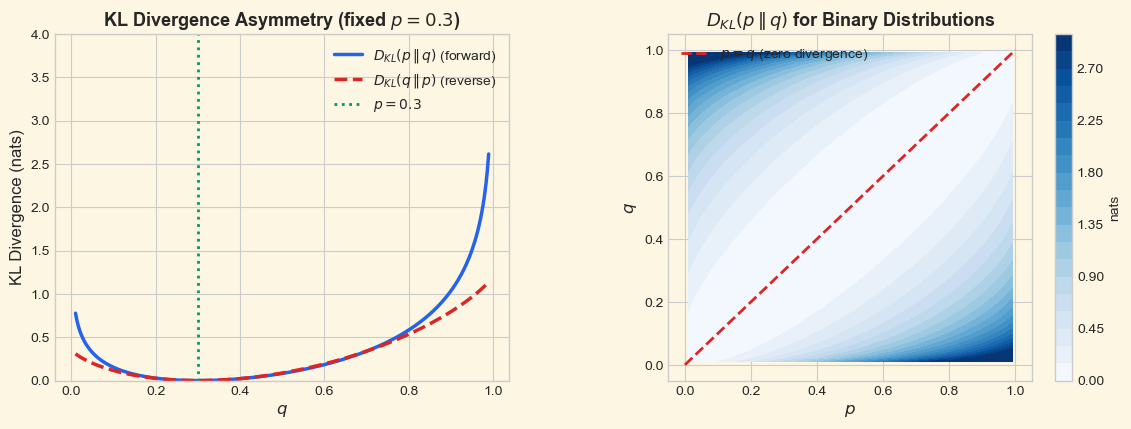
The left panel makes the asymmetry visually clear: the forward KL \(D_{\text{KL}}(p \,\|\, q)\) diverges to infinity as \(q \to 0\) (because \(p > 0\) there), while the reverse KL \(D_{\text{KL}}(q \,\|\, p)\) diverges as \(q \to 1\). Both are minimized (at zero) when \(q = p\).
26.3 Maximum Likelihood Estimation#
From Data to Models#
Suppose we observe data \(\{x_1, x_2, \ldots, x_N\}\) drawn independently from an unknown distribution \(p^*\). We have a parametric family of distributions \(\{p_\theta\}_{\theta \in \Theta}\) and wish to find the parameter \(\theta\) that best explains the data.
The likelihood of the data is:
The maximum likelihood estimator (MLE) is:
Ronald Fisher formalized this principle in 1922, though the idea of choosing parameters to maximize the probability of observed data can be traced back to Daniel Bernoulli (1778) and Johann Carl Friedrich Gauss, who used it to derive the method of least squares.
Theorem 26.4 (MLE Minimizes KL Divergence)
Maximum likelihood estimation is equivalent to minimizing the KL divergence \(D_{\text{KL}}(\hat{p}_{\text{data}} \,\|\, p_\theta)\), where \(\hat{p}_{\text{data}}\) is the empirical distribution of the data.
Proof
The empirical distribution assigns probability \(\hat{p}_{\text{data}}(x) = \frac{1}{N} \sum_{i=1}^{N} \mathbf{1}[x_i = x]\) to each observed value.
The KL divergence from the empirical distribution to the model is:
Expanding:
Since the first term does not depend on \(\theta\):
Now, substituting the empirical distribution:
This is precisely the negative log-likelihood (divided by \(N\)). Therefore:
This reveals the deep unity: MLE, cross-entropy minimization, and KL divergence minimization are all the same optimization problem. \(\blacksquare\)
The Big Picture
The three perspectives are equivalent when training a model \(q_\theta\) to match data from \(p\):
Perspective |
Objective |
Origin |
|---|---|---|
Maximum Likelihood |
\(\max_\theta \prod_i p_\theta(x_i)\) |
Fisher (1922) |
Cross-Entropy Minimization |
\(\min_\theta H(\hat{p}, p_\theta)\) |
Shannon (1948) |
KL Divergence Minimization |
\(\min_\theta D_{\text{KL}}(\hat{p} \,|\, p_\theta)\) |
Kullback & Leibler (1951) |
All three lead to the same \(\theta^*\). The differences are in interpretation, not in computation.
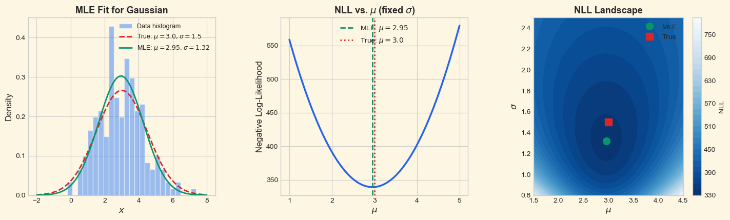
# MLE for a Gaussian: fit mean and variance to data
rng = np.random.default_rng(42)

# True parameters
true_mu = 3.0
true_sigma = 1.5
N = 200

# Generate data
data = rng.normal(loc=true_mu, scale=true_sigma, size=N)

# MLE estimates (for Gaussian, these are simply sample mean and sample std)
mu_mle = np.mean(data)
sigma_mle = np.std(data)  # MLE uses 1/N, not 1/(N-1)

print('Maximum Likelihood Estimation for Gaussian')
print('=' * 50)
print(f'True parameters:  mu = {true_mu:.4f}, sigma = {true_sigma:.4f}')
print(f'MLE estimates:    mu = {mu_mle:.4f}, sigma = {sigma_mle:.4f}')
print(f'Sample size:      N = {N}')
print()

# Compute negative log-likelihood for a grid of (mu, sigma) values
def neg_log_likelihood_gaussian(data, mu, sigma):
    """Negative log-likelihood of data under N(mu, sigma^2)."""
    n = len(data)
    return n/2 * np.log(2 * np.pi * sigma**2) + np.sum((data - mu)**2) / (2 * sigma**2)

nll_true = neg_log_likelihood_gaussian(data, true_mu, true_sigma)
nll_mle = neg_log_likelihood_gaussian(data, mu_mle, sigma_mle)
print(f'NLL at true params:  {nll_true:.4f}')
print(f'NLL at MLE params:   {nll_mle:.4f}')
print(f'MLE achieves lower NLL: {nll_mle < nll_true}')
Maximum Likelihood Estimation for Gaussian
==================================================
True parameters:  mu = 3.0000, sigma = 1.5000
MLE estimates:    mu = 2.9543, sigma = 1.3196
Sample size:      N = 200

NLL at true params:  342.3651
NLL at MLE params:   339.2516
MLE achieves lower NLL: True
Show code cell source
# Visualize MLE for Gaussian
fig, axes = plt.subplots(1, 3, figsize=(15, 4.5))
fig.patch.set_facecolor(CREAM)
for ax in axes:
    ax.set_facecolor(CREAM)

# Left: data histogram with fitted Gaussian
x_plot = np.linspace(-2, 8, 300)
pdf_true = (1 / (true_sigma * np.sqrt(2 * np.pi))) * \
    np.exp(-0.5 * ((x_plot - true_mu) / true_sigma) ** 2)
pdf_mle = (1 / (sigma_mle * np.sqrt(2 * np.pi))) * \
    np.exp(-0.5 * ((x_plot - mu_mle) / sigma_mle) ** 2)

axes[0].hist(data, bins=25, density=True, alpha=0.5, color=BLUE,
             edgecolor='white', label='Data histogram')
axes[0].plot(x_plot, pdf_true, color=RED, linewidth=2, linestyle='--',
             label=f'True: $\\mu={true_mu}, \\sigma={true_sigma}$')
axes[0].plot(x_plot, pdf_mle, color=GREEN, linewidth=2,
             label=f'MLE: $\\mu={mu_mle:.2f}, \\sigma={sigma_mle:.2f}$')
axes[0].set_xlabel('$x$', fontsize=12)
axes[0].set_ylabel('Density', fontsize=12)
axes[0].set_title('MLE Fit for Gaussian', fontsize=13, fontweight='bold')
axes[0].legend(fontsize=9)

# Middle: NLL as a function of mu (sigma fixed at MLE)
mu_range = np.linspace(1, 5, 200)
nll_mu = [neg_log_likelihood_gaussian(data, m, sigma_mle) for m in mu_range]

axes[1].plot(mu_range, nll_mu, color=DARK_BLUE, linewidth=2.5)
axes[1].axvline(x=mu_mle, color=GREEN, linestyle='--', linewidth=2,
                label=f'MLE: $\\mu = {mu_mle:.2f}$')
axes[1].axvline(x=true_mu, color=RED, linestyle=':', linewidth=2,
                label=f'True: $\\mu = {true_mu}$')
axes[1].set_xlabel('$\\mu$', fontsize=12)
axes[1].set_ylabel('Negative Log-Likelihood', fontsize=12)
axes[1].set_title('NLL vs. $\\mu$ (fixed $\\sigma$)', fontsize=13, fontweight='bold')
axes[1].legend(fontsize=10)

# Right: NLL contour plot over (mu, sigma)
mu_grid = np.linspace(1.5, 4.5, 100)
sigma_grid = np.linspace(0.8, 2.5, 100)
MU, SIGMA = np.meshgrid(mu_grid, sigma_grid)
NLL = np.zeros_like(MU)
for i in range(len(mu_grid)):
    for j in range(len(sigma_grid)):
        NLL[j, i] = neg_log_likelihood_gaussian(data, MU[j, i], SIGMA[j, i])

cs = axes[2].contourf(MU, SIGMA, NLL, levels=30, cmap='Blues_r')
axes[2].plot(mu_mle, sigma_mle, 'o', color=GREEN, markersize=10, zorder=5,
             label='MLE')
axes[2].plot(true_mu, true_sigma, 's', color=RED, markersize=10, zorder=5,
             label='True')
axes[2].set_xlabel('$\\mu$', fontsize=12)
axes[2].set_ylabel('$\\sigma$', fontsize=12)
axes[2].set_title('NLL Landscape', fontsize=13, fontweight='bold')
axes[2].legend(fontsize=10)
plt.colorbar(cs, ax=axes[2], label='NLL')

fig.subplots_adjust(left=0.05, right=0.95, wspace=0.35)
plt.show()
26.4 Cross-Entropy Loss for Classification#
From Theory to Practice#
In classification, the true label for sample \(i\) is a one-hot vector \(\mathbf{y}\) (e.g., \(\mathbf{y} = [0, 0, 1, 0]^\top\) for class 3 out of 4), and the network outputs predicted probabilities \(\hat{\mathbf{y}}\) via softmax. The categorical cross-entropy loss is:
Since \(\mathbf{y}\) is one-hot with \(y_c = 1\) for the correct class \(c\), this simplifies to:
This is exactly the negative log-likelihood of the correct class under the model’s predicted distribution, making cross-entropy loss a direct application of maximum likelihood estimation.
Binary Cross-Entropy#
For binary classification with a single sigmoid output \(\hat{y} = \sigma(z)\):
Why Cross-Entropy Beats MSE for Classification#
Consider a single sigmoid output \(\hat{y} = \sigma(z)\) for binary classification. The gradient of the loss with respect to the pre-activation \(z\) reveals a critical difference:
MSE loss \(L_{\text{MSE}} = \frac{1}{2}(\hat{y} - y)^2\):
The factor \(\sigma'(z) = \sigma(z)(1 - \sigma(z))\) vanishes when \(\sigma(z) \approx 0\) or \(\sigma(z) \approx 1\). This means when the network is confidently wrong, it learns very slowly (the sigmoid is saturated).
Cross-entropy loss \(L_{\text{CE}} = -[y \log \hat{y} + (1-y)\log(1-\hat{y})]\):
No \(\sigma'(z)\) factor! The gradient is proportional to the error alone. When the network is confidently wrong, the gradient is large, providing a strong learning signal. This was one of the key insights that made backpropagation practical for classification (Rumelhart, Hinton & Williams, 1986).
Key Insight
Cross-entropy loss “cancels out” the saturation of the sigmoid/softmax activation. The gradient \(\partial L / \partial z = \hat{y} - y\) is simple, bounded, and never vanishes—it provides a learning signal proportional to the prediction error.
Theorem 26.5 (Softmax + Cross-Entropy Gradient)
For a network with softmax output \(\hat{y}_k = \frac{e^{z_k}}{\sum_j e^{z_j}}\) and cross-entropy loss \(L = -\sum_k y_k \log \hat{y}_k\), the gradient with respect to the pre-softmax logit \(z_j\) is:
Proof
We need \(\frac{\partial L}{\partial z_j} = -\sum_k y_k \frac{\partial \log \hat{y}_k}{\partial z_j} = -\sum_k y_k \frac{1}{\hat{y}_k} \frac{\partial \hat{y}_k}{\partial z_j}.\)
First, we compute the softmax Jacobian. Let \(S = \sum_m e^{z_m}\).
Case 1: \(k = j\).
Case 2: \(k \neq j\).
Combining with the Kronecker delta: \(\frac{\partial \hat{y}_k}{\partial z_j} = \hat{y}_k(\delta_{kj} - \hat{y}_j).\)
Now substituting into the loss gradient:
Expanding:
where we used \(\sum_k y_k = 1\) (since \(\mathbf{y}\) is one-hot). \(\blacksquare\)
def sigmoid(z):
    """Numerically stable sigmoid function."""
    return np.where(z >= 0,
                    1 / (1 + np.exp(-z)),
                    np.exp(z) / (1 + np.exp(z)))


def binary_cross_entropy(y, y_hat):
    """Binary cross-entropy loss.

    Parameters
    ----------
    y : float or array
        True label (0 or 1).
    y_hat : float or array
        Predicted probability.

    Returns
    -------
    float or array
        Binary cross-entropy loss.
    """
    eps = 1e-15  # Prevent log(0)
    y_hat = np.clip(y_hat, eps, 1 - eps)
    return -(y * np.log(y_hat) + (1 - y) * np.log(1 - y_hat))


def categorical_cross_entropy(y_onehot, y_hat):
    """Categorical cross-entropy loss.

    Parameters
    ----------
    y_onehot : array, shape (K,)
        One-hot encoded true label.
    y_hat : array, shape (K,)
        Predicted probabilities (must sum to 1).

    Returns
    -------
    float
        Cross-entropy loss.
    """
    eps = 1e-15
    y_hat = np.clip(y_hat, eps, 1.0)
    return -np.sum(y_onehot * np.log(y_hat))


# Demonstrate: CE loss for correct vs incorrect predictions
print('Cross-Entropy Loss Examples')
print('=' * 55)
print(f'{"Prediction":>30s}  {"True":>8s}  {"CE Loss":>8s}')
print('-' * 55)

examples = [
    ([0.9, 0.05, 0.05], [1, 0, 0], 'Confident & correct'),
    ([0.6, 0.2, 0.2], [1, 0, 0], 'Uncertain & correct'),
    ([0.33, 0.34, 0.33], [1, 0, 0], 'Near-uniform'),
    ([0.1, 0.8, 0.1], [1, 0, 0], 'Confident & wrong'),
    ([0.01, 0.01, 0.98], [1, 0, 0], 'Very wrong'),
]

for y_hat, y_true, desc in examples:
    loss = categorical_cross_entropy(np.array(y_true), np.array(y_hat))
    print(f'{desc:>30s}  {str(y_true):>8s}  {loss:>8.4f}')
Cross-Entropy Loss Examples
=======================================================
                    Prediction      True   CE Loss
-------------------------------------------------------
           Confident & correct  [1, 0, 0]    0.1054
           Uncertain & correct  [1, 0, 0]    0.5108
                  Near-uniform  [1, 0, 0]    1.1087
             Confident & wrong  [1, 0, 0]    2.3026
                    Very wrong  [1, 0, 0]    4.6052
Show code cell source
# Compare MSE vs CE gradient magnitude for sigmoid output
fig, axes = plt.subplots(1, 3, figsize=(15, 4.5))
fig.patch.set_facecolor(CREAM)
for ax in axes:
    ax.set_facecolor(CREAM)

z_range = np.linspace(-6, 6, 500)
y_hat = sigmoid(z_range)
sigma_prime = y_hat * (1 - y_hat)

# For y = 1 (true label is positive)
y = 1.0

# MSE gradient w.r.t. z: (y_hat - y) * sigma'(z)
grad_mse = (y_hat - y) * sigma_prime

# CE gradient w.r.t. z: (y_hat - y)
grad_ce = y_hat - y

# Left: loss curves
loss_mse = 0.5 * (y_hat - y) ** 2
loss_ce = binary_cross_entropy(y, y_hat)

axes[0].plot(z_range, loss_mse, color=RED, linewidth=2.5, label='MSE loss')
axes[0].plot(z_range, loss_ce, color=DARK_BLUE, linewidth=2.5, label='CE loss')
axes[0].set_xlabel('Pre-activation $z$', fontsize=12)
axes[0].set_ylabel('Loss', fontsize=12)
axes[0].set_title('MSE vs. CE Loss ($y = 1$)', fontsize=13, fontweight='bold')
axes[0].legend(fontsize=11)
axes[0].set_ylim(0, 5)

# Middle: gradient magnitude
axes[1].plot(z_range, np.abs(grad_mse), color=RED, linewidth=2.5,
             label=r'MSE: $|(\hat{y}-y)\sigma\'(z)|$')
axes[1].plot(z_range, np.abs(grad_ce), color=DARK_BLUE, linewidth=2.5,
             label=r'CE: $|\hat{y}-y|$')
axes[1].set_xlabel('Pre-activation $z$', fontsize=12)
axes[1].set_ylabel(r'$|\partial L / \partial z|$', fontsize=12)
axes[1].set_title('Gradient Magnitude ($y = 1$)', fontsize=13, fontweight='bold')
axes[1].legend(fontsize=10)
axes[1].set_ylim(0, 1.2)

# Annotate the saturation problem
axes[1].annotate('Sigmoid\nsaturated!',
                 xy=(-5, np.abs((sigmoid(-5) - 1) * sigmoid(-5) * (1-sigmoid(-5)))),
                 xytext=(-4, 0.6),
                 fontsize=10, color=RED, fontweight='bold',
                 arrowprops=dict(arrowstyle='->', color=RED, lw=1.5))

# Right: sigmoid and its derivative
axes[2].plot(z_range, y_hat, color=DARK_BLUE, linewidth=2.5, label=r'$\sigma(z)$')
axes[2].plot(z_range, sigma_prime, color=AMBER, linewidth=2.5, linestyle='--',
             label=r"$\sigma'(z)$")
axes[2].axhline(y=0.25, color='gray', linestyle=':', alpha=0.5)
axes[2].set_xlabel('$z$', fontsize=12)
axes[2].set_ylabel('Value', fontsize=12)
axes[2].set_title(r'Sigmoid and Its Derivative', fontsize=13, fontweight='bold')
axes[2].legend(fontsize=11)

plt.tight_layout()
plt.show()
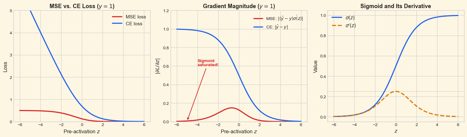
The middle panel shows the key result: the MSE gradient (red) nearly vanishes for large negative \(z\) (where \(\sigma(z) \approx 0\)), precisely the region where the network is confidently wrong and most needs to learn. The CE gradient (blue) remains strong throughout, proportional to the prediction error.
26.5 Softmax as a Boltzmann Distribution#
From Statistical Mechanics to Neural Networks#
The softmax function used in neural network outputs has deep roots in statistical mechanics. Ludwig Boltzmann (1868) and Josiah Willard Gibbs (1902) showed that in thermal equilibrium, the probability of a physical system being in state \(k\) with energy \(E_k\) at temperature \(T\) is:
where \(k_B\) is Boltzmann’s constant and the denominator \(Z = \sum_j e^{-E_j / (k_B T)}\) is the partition function.
In neural networks, we identify the negative logit \(-z_k\) with energy (or equivalently, \(z_k\) with negative energy), giving the softmax with temperature:
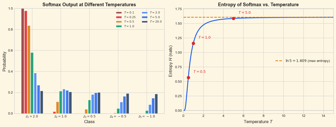
The standard softmax uses \(T = 1\). The temperature \(T\) controls the “sharpness” of the distribution:
\(T \to 0\) (low temperature): the distribution concentrates on the state with the highest logit (approaches argmax / hard decision).
\(T = 1\) (standard): the usual softmax.
\(T \to \infty\) (high temperature): all states become equally likely (approaches uniform distribution / maximum entropy).
This connection was made explicit in neural networks through Geoffrey Hinton’s Boltzmann machines (Ackley, Hinton & Sejnowski, 1985), which used stochastic units with Boltzmann-distributed activations. Temperature scaling has recently found renewed importance in knowledge distillation (Hinton et al., 2015) and language model sampling.
Temperature and Entropy
As \(T\) increases, the entropy of the softmax output increases, reaching maximum entropy (\(\ln K\) for \(K\) classes) as \(T \to \infty\). As \(T\) decreases toward zero, the entropy decreases toward zero (a deterministic distribution). Temperature thus provides a smooth interpolation between maximum confidence and maximum uncertainty.
Show code cell source
def softmax(z, temperature=1.0):
    """Numerically stable softmax with temperature."""
    z_scaled = z / temperature
    z_shifted = z_scaled - np.max(z_scaled)  # Numerical stability
    exp_z = np.exp(z_shifted)
    return exp_z / np.sum(exp_z)


# Demonstrate softmax with different temperatures
logits = np.array([2.0, 1.0, 0.5, -0.5, -1.0])
temperatures = [0.1, 0.25, 0.5, 1.0, 2.0, 5.0, 20.0]

fig, axes = plt.subplots(1, 2, figsize=(13, 5))
fig.patch.set_facecolor(CREAM)
for ax in axes:
    ax.set_facecolor(CREAM)

# Left: bar chart for different temperatures
n_classes = len(logits)
x_pos = np.arange(n_classes)
width = 0.11
colors_temp = [BURGUNDY, RED, AMBER, GREEN, BLUE, DARK_BLUE, '#1e3a5f']

for idx, T in enumerate(temperatures):
    probs = softmax(logits, temperature=T)
    offset = (idx - len(temperatures) / 2 + 0.5) * width
    axes[0].bar(x_pos + offset, probs, width * 0.9, color=colors_temp[idx],
                alpha=0.85, label=f'$T = {T}$', edgecolor='white')

axes[0].set_xlabel('Class', fontsize=12)
axes[0].set_ylabel('Probability', fontsize=12)
axes[0].set_title('Softmax Output at Different Temperatures',
                   fontsize=13, fontweight='bold')
axes[0].set_xticks(x_pos)
axes[0].set_xticklabels([f'$z_{k+1}={logits[k]:.1f}$' for k in range(n_classes)],
                         fontsize=9)
axes[0].legend(fontsize=8, ncol=2, loc='upper right')
axes[0].set_ylim(0, 1.0)

# Right: entropy of softmax output vs temperature
temp_range = np.linspace(0.05, 15, 300)
entropies = [entropy(softmax(logits, T)) for T in temp_range]

axes[1].plot(temp_range, entropies, color=DARK_BLUE, linewidth=2.5)
axes[1].axhline(y=np.log(n_classes), color=AMBER, linestyle='--', linewidth=2,
                label=f'$\\ln {n_classes} = {np.log(n_classes):.3f}$ (max entropy)')
axes[1].axhline(y=0, color='gray', linestyle=':', alpha=0.5)

# Mark specific temperatures
for T_mark in [0.5, 1.0, 5.0]:
    h_mark = entropy(softmax(logits, T_mark))
    axes[1].plot(T_mark, h_mark, 'o', color=RED, markersize=8, zorder=5)
    axes[1].annotate(f'$T={T_mark}$', xy=(T_mark, h_mark),
                     xytext=(T_mark + 0.5, h_mark + 0.08),
                     fontsize=10, color=RED)

axes[1].set_xlabel('Temperature $T$', fontsize=12)
axes[1].set_ylabel('Entropy $H$ (nats)', fontsize=12)
axes[1].set_title('Entropy of Softmax vs. Temperature',
                   fontsize=13, fontweight='bold')
axes[1].legend(fontsize=10)
axes[1].set_xlim(0, 15)
axes[1].set_ylim(-0.05, np.log(n_classes) + 0.15)

plt.tight_layout()
plt.show()
Show code cell source
# Demonstrate softmax temperature in a 2D classification landscape
fig, axes = plt.subplots(1, 3, figsize=(15, 4.5))
fig.patch.set_facecolor(CREAM)

# Create a simple 3-class problem with logits as a function of position
x_grid = np.linspace(-3, 3, 200)
y_grid = np.linspace(-3, 3, 200)
X, Y = np.meshgrid(x_grid, y_grid)

# Three class centers
centers = np.array([[1.5, 1.5], [-1.5, 1.0], [0.0, -1.5]])
class_colors = [BLUE, GREEN, AMBER]

temp_vals = [0.3, 1.0, 5.0]
temp_labels = ['Low ($T = 0.3$)', 'Standard ($T = 1.0$)', 'High ($T = 5.0$)']

for ax_idx, (T, label) in enumerate(zip(temp_vals, temp_labels)):
    ax = axes[ax_idx]
    ax.set_facecolor(CREAM)

    # Compute logits as negative distance to each center
    probs = np.zeros((*X.shape, 3))
    for i in range(X.shape[0]):
        for j in range(X.shape[1]):
            point = np.array([X[i, j], Y[i, j]])
            logits_ij = -np.array([np.linalg.norm(point - c) for c in centers])
            probs[i, j] = softmax(logits_ij, temperature=T)

    # Create RGB image from class probabilities
    # Map: class 0 -> blue, class 1 -> green, class 2 -> amber
    rgb_colors = np.array([
        [59/255, 130/255, 246/255],   # blue
        [5/255, 150/255, 105/255],    # green
        [217/255, 119/255, 6/255],    # amber
    ])

    img = np.einsum('ijk,kl->ijl', probs, rgb_colors)
    img = np.clip(img, 0, 1)

    ax.imshow(img, extent=[-3, 3, -3, 3], origin='lower', aspect='equal')
    for k, c in enumerate(centers):
        ax.plot(c[0], c[1], 'o', color='white', markersize=12,
                markeredgecolor='black', markeredgewidth=2)
        ax.annotate(f'Class {k+1}', xy=(c[0], c[1]),
                    xytext=(c[0]+0.3, c[1]+0.3), fontsize=9,
                    color='white', fontweight='bold',
                    bbox=dict(boxstyle='round,pad=0.2', facecolor='black', alpha=0.5))

    e_val = np.mean([entropy(probs[i, j]) for i in range(0, 200, 10)
                      for j in range(0, 200, 10)])
    ax.set_title(f'{label}\nMean entropy: {e_val:.3f}',
                 fontsize=12, fontweight='bold')
    ax.set_xlabel('$x_1$', fontsize=11)
    if ax_idx == 0:
        ax.set_ylabel('$x_2$', fontsize=11)

plt.suptitle('Decision Boundaries at Different Temperatures',
             fontsize=14, fontweight='bold', y=1.02)
plt.tight_layout(rect=[0, 0, 1, 0.93])
plt.show()

At low temperature (\(T = 0.3\)), the softmax output is nearly deterministic: each point is assigned almost entirely to the nearest class, producing sharp decision boundaries. At high temperature (\(T = 5.0\)), the probabilities are nearly uniform everywhere—the model “hedges its bets.” Standard temperature (\(T = 1.0\)) provides a smooth interpolation that preserves the relative ordering of logits while expressing genuine uncertainty near decision boundaries.
Exercises#
Exercise 26.1. Compute the entropy of the following distributions and rank them from lowest to highest entropy: (a) \(p = (1/2, 1/4, 1/8, 1/8)\), (b) \(p = (1/4, 1/4, 1/4, 1/4)\), © \(p = (1, 0, 0, 0)\), (d) \(p = (1/3, 1/3, 1/6, 1/6)\). Verify your answers computationally.
Exercise 26.2. Prove that \(D_{\text{KL}}(p \,\|\, q) = 0\) implies \(p = q\) (the strict equality case of Gibbs’ inequality) without using Jensen’s inequality. Hint: use the inequality \(\ln x \leq x - 1\) with equality iff \(x = 1\).
Exercise 26.3. Consider a coin with unknown bias \(\theta\) (probability of heads). You observe the sequence HHTHT (3 heads, 2 tails). (a) Write down the likelihood \(\mathcal{L}(\theta)\) and log-likelihood \(\ell(\theta)\). (b) Find \(\hat{\theta}_{\text{MLE}}\) by setting \(\ell'(\theta) = 0\). © Plot the log-likelihood as a function of \(\theta\) and verify your answer.
Exercise 26.4. Derive the gradient \(\frac{\partial L_{\text{BCE}}}{\partial z}\) for binary cross-entropy with sigmoid output \(\hat{y} = \sigma(z)\), showing explicitly how the \(\sigma'(z)\) term cancels. Compare with the MSE gradient.
Exercise 26.5. The Jensen-Shannon divergence is defined as: $\(D_{\text{JS}}(p \,\|\, q) = \frac{1}{2} D_{\text{KL}}\!\left(p \,\Big\|\, \frac{p+q}{2}\right) + \frac{1}{2} D_{\text{KL}}\!\left(q \,\Big\|\, \frac{p+q}{2}\right).\)\( (a) Prove that \)D_{\text{JS}}(p ,|, q) = D_{\text{JS}}(q ,|, p)\( (symmetry). (b) Prove that \)0 \leq D_{\text{JS}}(p ,|, q) \leq \ln 2$. © Implement the JS divergence and verify numerically that it is symmetric for several example distributions.
Exercise 26.6. Show that as the temperature \(T \to 0^+\), the softmax function \(\hat{y}_k = \frac{e^{z_k/T}}{\sum_j e^{z_j/T}}\) converges to a one-hot vector with \(\hat{y}_{k^*} = 1\) where \(k^* = \arg\max_k z_k\) (assuming a unique maximum). Hint: factor out \(e^{z_{k^*}/T}\) from numerator and denominator.