Chapter 50: Regev’s LWE — From LPN to a Public-Key Cryptosystem#
This chapter walks you through Oded Regev’s 2005 paper On Lattices, Learning with Errors, Random Linear Codes, and Cryptography (STOC ‘05; Journal of the ACM 56(6), 2009) — the paper that introduced the Learning with Errors (LWE) problem and the first cryptosystem provably as hard to break as worst-case lattice problems.
Source PDF: sources/1060590.1060603.pdf in this repo.
The plan:
§ |
What |
|---|---|
50.1 |
Roadmap |
50.2 |
The simple problem — Learning Parity with Noise (LPN) mod 2 |
50.3 |
Generalise to LWE mod \(p\) |
50.4 |
Two equivalent views: CVP on a \(q\)-ary lattice, decoding a random code |
50.5 |
Theorem 1.1 — the quantum worst-case to average-case reduction |
50.6 |
The public-key cryptosystem (Section 4 of the paper) |
50.7 |
Closing notes: from Regev 2005 to ML-KEM (2024) |
Every section has runnable Python — the same data structures recur from Part I to Part VI, so when you get to the cryptosystem you are not seeing it for the first time.
Why this tutorial sits here
The post-quantum standards ML-KEM (FIPS 203) and ML-DSA (FIPS 204) are direct descendants of Regev’s construction. Understanding Section 4 of his 2005 paper is the cleanest way to get the “why” of every design choice in Kyber. You have already covered the quantum half of the course, so the quantum step in Theorem 1.1’s proof will be natural.
50.1 Roadmap#
The story arc has four characters:
LPN (\(p = 2\)). The “learning parity with noise” problem: given many noisy parity equations \(\langle \mathbf{s}, \mathbf{a}_i\rangle = b_i \pmod 2\) that hold with some probability \(1-\varepsilon\), recover the secret \(\mathbf{s} \in \mathbb{F}_2^n\). Without noise this is trivial Gaussian elimination; with noise it is believed hard (best-known algorithm runs in time \(2^{O(n/\log n)}\), Blum–Kalai–Wasserman 2003).
LWE (\(p > 2\)). The same equations, but modulo a polynomial-sized prime \(p\) and with errors drawn from a (discretised) Gaussian. The change of modulus is what enables Regev’s quantum reduction.
Theorem 1.1. Solving LWE on average is at least as hard as worst-case approximate-SVP on every \(n\)-dimensional lattice — but only via a quantum algorithm. A classical worst-case ↔ average-case reduction for LWE was later obtained by Peikert (2009) for restricted parameters, and extended by Brakerski–Langlois–Peikert–Regev–Stehlé (2013) to a wider regime; neither result quite recovers Theorem 1.1’s full strength classically.
The cryptosystem. A few-line public-key scheme whose IND-CPA security reduces to LWE. Encryption blows up message length by \(O(\log p)\), decryption rounds to the nearest of two integer buckets.
Notation we will use throughout
\(n\) — security parameter (lattice / secret dimension).
\(p\) — a prime modulus, polynomial in \(n\) (in the cryptosystem \(n^2 \le p \le 2n^2\)).
\(\mathbf{s} \in \mathbb{Z}_p^n\) — the secret.
\(\mathbf{a}_i \in \mathbb{Z}_p^n\) — the public “queries”, uniform.
\(e_i \in \mathbb{Z}_p\) — small errors.
\(b_i := \langle \mathbf{a}_i, \mathbf{s}\rangle + e_i \pmod p\).
\(\chi\) — error distribution (in LWE we use \(\bar\Psi_\alpha\), a discretised Gaussian on \(\mathbb{Z}_p\) with parameter \(\alpha p\)).
\(m\) — number of LWE samples used in the public key. In the cryptosystem \(m = 5n\).
50.2 The simple problem — Learning Parity with Noise (LPN)#
Definition — LPN(\(n, \varepsilon\))
Fix a secret \(\mathbf{s} \in \mathbb{F}_2^n\). Each LPN sample is a pair \((\mathbf{a}_i, b_i) \in \mathbb{F}_2^n \times \mathbb{F}_2\) where \(\mathbf{a}_i\) is uniform and
The LPN problem is: given polynomially many samples, recover \(\mathbf{s}\).
The case \(\varepsilon = 0\) is trivial: gather \(n\) linearly-independent samples, write them as a matrix equation \(A\mathbf{s} = \mathbf{b}\), solve by Gaussian elimination — \(O(n^3)\) time.
The moment \(\varepsilon > 0\) the problem looks completely different: flipping a single bit of \(A\mathbf{s}\) propagates through Gaussian elimination and contaminates every row of the result. Even with the best-known algorithm (Blum–Kalai–Wasserman) the cost is sub-exponential \(2^{O(n/\log n)}\).
50.2.1 Build an LPN sampler — Exercise#
Implement an lpn_sample(s, eps, rng) helper that returns one
\((\mathbf{a}, b)\) pair. Use it to generate \(m\) samples for a small
example and verify the noise empirically.
import numpy as np

def lpn_sample(s, eps, rng):
    '''One LPN sample (a, b) with s in F_2^n, b = <a, s> + e mod 2,  P(e=1)=eps.'''
    n = len(s)
    a = rng.integers(0, 2, size=n)
    b = (int(a @ s) + int(rng.random() < eps)) % 2
    return a, b


# Demo: n = 6, eps = 0.1, m = 1000 samples.
rng = np.random.default_rng(20260519)
n, eps, m = 6, 0.1, 1000
s_true = rng.integers(0, 2, size=n)

A = np.zeros((m, n), dtype=int)
b = np.zeros(m, dtype=int)
for i in range(m):
    A[i], b[i] = lpn_sample(s_true, eps, rng)

# Empirical noise rate = fraction of rows where <a_i, s_true> != b_i.
predicted = (A @ s_true) % 2
empirical_eps = float(np.mean(predicted != b))
print(f'Secret    s = {s_true.tolist()}')
print(f'Samples   m = {m},  n = {n},  target eps = {eps}')
print(f'Empirical eps = {empirical_eps:.3f}   (should be close to {eps})')
Secret    s = [1, 0, 0, 1, 0, 1]
Samples   m = 1000,  n = 6,  target eps = 0.1
Empirical eps = 0.088   (should be close to 0.1)
50.2.2 The \(\varepsilon = 0\) case — Gaussian elimination over \(\mathbb{F}_2\)#
When the noise rate is zero, every equation is exact, and any \(n\) linearly-independent samples uniquely determine the secret.
def gauss_solve_f2(A, b):
    '''Solve A s = b over F_2 for square invertible A.  Returns s or None.'''
    n = len(b)
    M = np.hstack([A.copy() % 2, b.reshape(-1, 1) % 2])
    row = 0
    for col in range(n):
        # find pivot
        piv = None
        for r in range(row, M.shape[0]):
            if M[r, col]:
                piv = r; break
        if piv is None:
            continue
        M[[row, piv]] = M[[piv, row]]
        # eliminate other rows
        for r in range(M.shape[0]):
            if r != row and M[r, col]:
                M[r] = (M[r] + M[row]) % 2
        row += 1
    if row < n:
        return None
    # back-substitute
    return M[:n, -1] % 2


# Verify Gaussian elimination on a noise-free instance.
rng = np.random.default_rng(7)
s_true = rng.integers(0, 2, size=8)
A = rng.integers(0, 2, size=(8, 8))
while int(round(np.linalg.det(A.astype(float))) % 2) == 0:
    A = rng.integers(0, 2, size=(8, 8))
b = (A @ s_true) % 2
s_rec = gauss_solve_f2(A, b)
print(f'noise-free recovery: rec = {s_rec.tolist()},  true = {s_true.tolist()},  match = {np.array_equal(s_rec, s_true)}')

# Now break Gaussian elimination by flipping one bit of b.
b_noisy = b.copy(); b_noisy[3] ^= 1
s_wrong = gauss_solve_f2(A, b_noisy)
print(f'one-bit error      : rec = {s_wrong.tolist()},  matches in {int(np.sum(s_wrong == s_true))}/{len(s_true)} positions')
noise-free recovery: rec = [1, 1, 1, 1, 1, 1, 1, 0],  true = [1, 1, 1, 1, 1, 1, 1, 0],  match = True
one-bit error      : rec = [0, 1, 0, 0, 1, 0, 1, 1],  matches in 3/8 positions
Notice what happens with a single flipped bit: Gaussian elimination propagates the error, and the recovered “secret” disagrees with the true one in many positions. This is the qualitative phenomenon that makes LPN/LWE so much harder than its noise-free cousin.
50.2.3 Naive maximum-likelihood — Exercise#
A textbook attack is the maximum-likelihood (ML) estimator: try every \(\mathbf{s} \in \mathbb{F}_2^n\) and pick the one minimising the number of “wrong” equations. Run-time: \(2^n\).
This is impractical for cryptographic \(n\) but a useful sanity check for tiny \(n\).
import itertools

def lpn_ml_attack(A, b):
    '''Maximum-likelihood attack: try every secret, return the one matching most equations.'''
    n = A.shape[1]
    best_s, best_disagreements = None, len(b) + 1
    for bits in itertools.product([0, 1], repeat=n):
        s = np.array(bits, dtype=int)
        pred = (A @ s) % 2
        d = int(np.sum(pred != b))
        if d < best_disagreements:
            best_disagreements = d; best_s = s
    return best_s, best_disagreements


# Run on our (n=6, eps=0.1, m=1000) instance from above.
s_rec, dis = lpn_ml_attack(A[:500], b[:500])    # use first 500 samples
print(f'ML attack recovered s = {s_rec.tolist()}   disagreements = {dis} / 500')
print(f'Matches true s ?       {np.array_equal(s_rec, s_true[:6] if len(s_true)>=6 else s_true)}')

# Re-run on the real LPN instance (n=6).
rng = np.random.default_rng(20260519)
s_true = rng.integers(0, 2, size=6)
m = 1000; eps = 0.1
A = np.zeros((m, 6), dtype=int); b = np.zeros(m, dtype=int)
for i in range(m):
    A[i], b[i] = lpn_sample(s_true, eps, rng)
s_rec, dis = lpn_ml_attack(A, b)
print(f'LPN(n=6, eps=0.1)      true s = {s_true.tolist()}   rec s = {s_rec.tolist()}   match = {np.array_equal(s_rec, s_true)}')
print(f'Total disagreements = {dis} / {m}   (expected ~{eps*m:.0f})')
ML attack recovered s = [1, 1, 1, 1, 1, 1, 1, 0]   disagreements = 0 / 500
Matches true s ?       False
LPN(n=6, eps=0.1)      true s = [1, 0, 0, 1, 0, 1]   rec s = [1, 0, 0, 1, 0, 1]   match = True
Total disagreements = 88 / 1000   (expected ~100)
Why this scales so badly
The ML attack runs in \(\Theta(2^n \cdot m)\) time. For LPN at \(n = 64\) the brute force is \(\approx 10^{19} \cdot m\) — infeasible. Beating brute-force is non-trivial; the best generic attack remains Blum–Kalai–Wasserman 2003, which uses cleverly-chosen subset sums of samples to reduce the effective dimension, costing \(2^{O(n/\log n)}\). That is sub-exponential but still exponential in \(n / \log n\).
That is the punch line of §50.2: adding noise makes a polynomial problem sub-exponential. Regev’s contribution starts by asking what happens when we change the modulus from 2 to a polynomial-size prime.
50.3 Generalising to LWE#
Definition — LWE\(_{p,\chi}\)
Fix:
a security parameter \(n\),
a prime modulus \(p = p(n)\), polynomial in \(n\),
an error distribution \(\chi\) on \(\mathbb{Z}_p\) (a “small” distribution),
a secret \(\mathbf{s} \in \mathbb{Z}_p^n\).
An LWE sample is a pair \((\mathbf{a}_i, b_i) \in \mathbb{Z}_p^n \times \mathbb{Z}_p\) with \(\mathbf{a}_i\) uniform and
LWE\(_{p,\chi}\) asks: given polynomially many samples, recover \(\mathbf{s}\).
Regev fixes \(\chi = \bar\Psi_\alpha\), where \(\bar\Psi_\alpha\) is the discretised periodic Gaussian on \(\mathbb{Z}_p\) with parameter \(\alpha\). Operationally:
sample \(r \sim \mathcal{N}(0, (\alpha)^2)\), reduce \(r\) mod 1 (periodise to \(\mathbb{T} = \mathbb{R}/\mathbb{Z}\)), then round \(p \cdot r\) to the nearest integer in \(\mathbb{Z}_p\).
For typical parameters \(\alpha\) is set so the standard deviation of \(\alpha p\) is much smaller than \(p/2\) — small enough that decryption works, large enough that LWE remains hard.
50.3.1 Build the LWE sampler — Exercise#
def psi_bar_alpha(alpha, p, rng, size=None):
    '''Discretised periodic Gaussian on Z_p.  Following Regev (2005) Section 2:
    Psi_beta samples a real r ~ N(0, (beta/sqrt(2 pi))^2) and reduces mod 1.
    Psi_bar_beta further discretises by multiplying by p and rounding to Z_p.
    The resulting standard deviation on Z_p (centred) is approximately
    alpha * p / sqrt(2 pi).
    '''
    sigma_T = alpha / np.sqrt(2 * np.pi)
    r = rng.normal(0.0, sigma_T, size=size)
    r_mod1 = r - np.floor(r + 0.5)                   # reduce to (-1/2, 1/2]
    return np.round(p * r_mod1).astype(int) % p      # discretise to Z_p (centred lift)


def lwe_sample(s, p, alpha, rng):
    '''One LWE sample (a, b) with b = <a, s> + e mod p, e ~ psi_bar_alpha.'''
    n = len(s)
    a = rng.integers(0, p, size=n)
    e = int(psi_bar_alpha(alpha, p, rng))
    b = (int(a @ s) + e) % p
    return a, b


# Demo: n=4, p=97, alpha=0.05.  Visualise the error empirically.
import matplotlib.pyplot as plt
rng = np.random.default_rng(2026)
n, p, alpha, m = 4, 97, 0.05, 5000
s = rng.integers(0, p, size=n)

A = np.zeros((m, n), dtype=int); b = np.zeros(m, dtype=int)
for i in range(m):
    A[i], b[i] = lwe_sample(s, p, alpha, rng)

# Recover errors: e_i = (b_i - <a_i, s>) mod p, lifted to (-p/2, p/2].
errors = (b - (A @ s)) % p
errors_centred = np.where(errors > p // 2, errors - p, errors)

print(f'Secret s    = {s.tolist()}')
print(f'Empirical error sd = {float(np.std(errors_centred)):.3f}   (theory ~ alpha*p/sqrt(2*pi) = {alpha*p/np.sqrt(2*np.pi):.3f})')
print(f'Error range = [{int(errors_centred.min())}, {int(errors_centred.max())}]   (vs p/2 = {p//2})')

# Histogram of centred errors.
fig, ax = plt.subplots(figsize=(7, 3.5))
ax.hist(errors_centred, bins=range(int(errors_centred.min()) - 1, int(errors_centred.max()) + 2),
        color='steelblue', edgecolor='navy', alpha=0.8, density=True)
xs = np.linspace(errors_centred.min() - 1, errors_centred.max() + 1, 200)
sigma = alpha * p
ax.plot(xs, np.exp(-xs**2 / (2 * sigma**2)) / (sigma * np.sqrt(2 * np.pi)),
        'r-', lw=2, label=fr'$\mathcal{{N}}(0,\,(\alpha p)^2)$ with $\alpha p = {sigma:.2f}$')
ax.set_xlabel(r'centred error  $e_i$', fontsize=11)
ax.set_ylabel('density', fontsize=11)
ax.set_title(r'$\bar\Psi_\alpha$ noise (centred); $p=$' + f'{p}, $\\alpha=${alpha}', fontsize=12)
ax.legend(); ax.grid(True, alpha=0.3)
plt.tight_layout(); plt.show()
Secret s    = [82, 17, 2, 62]
Empirical error sd = 1.956   (theory ~ alpha*p/sqrt(2*pi) = 1.935)
Error range = [-7, 7]   (vs p/2 = 48)

50.3.2 Visualise samples in the \((a, b)\) plane#
When \(n = 1\), every sample is a 2-D point \((a, b) \in \mathbb{Z}_p^2\) — ideal for a picture. The “ideal” (zero-error) samples lie exactly on the line \(b = s \cdot a \pmod p\); the noise jitters each sample vertically by an amount drawn from \(\bar\Psi_\alpha\).
rng = np.random.default_rng(11)
p, alpha = 23, 0.04
s_scalar = 7                                                # the 1-D secret
n_samples = 60

a = rng.integers(0, p, size=n_samples)
e = psi_bar_alpha(alpha, p, rng, size=n_samples)
b = (a * s_scalar + e) % p

fig, ax = plt.subplots(figsize=(7, 6))
# Draw the noiseless line  b = s*a mod p, plus its periodic shifts +/- p.
xs = np.arange(p + 1)
for shift in (-1, 0, 1):
    ax.plot(xs, xs * s_scalar + shift * p, 'b:', alpha=0.4, lw=1)
# Draw the samples.
ax.scatter(a, b, c='red', marker='*', s=70, zorder=5,
           label=fr'LWE samples (errors $e_i \sim \bar\Psi_{{{alpha}}}$)')
ax.set_xlim(-1, p + 0.5); ax.set_ylim(-2, p + 1)
ax.set_xlabel('a'); ax.set_ylabel('b')
ax.set_title(fr'LWE with $n=1$, $p={p}$, secret $s={s_scalar}$  ' +
             r'($b = s\,a + e \;\mathrm{mod}\; p$)')
ax.grid(True, alpha=0.3); ax.legend(loc='upper left')
plt.tight_layout(); plt.show()

print(f'true secret s = {s_scalar}')
print(f'first 8 samples (a, b):  {list(zip(a[:8].tolist(), b[:8].tolist()))}')

true secret s = 7
first 8 samples (a, b):  [(3, 21), (2, 14), (18, 11), (11, 8), (13, 22), (13, 22), (16, 20), (0, 0)]
50.4 Two equivalent views#
LWE is the same problem in three guises. Recognising each makes the later proofs and parameter choices easier to read.
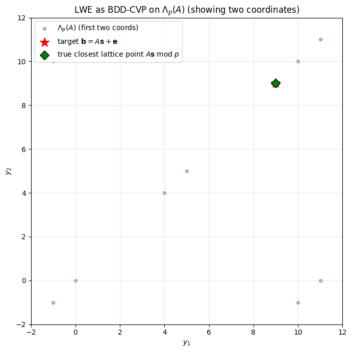
50.4.1 View A — LWE as Bounded-Distance CVP on a \(q\)-ary lattice#
Stack \(m\) samples as \((A, \mathbf{b}) \in \mathbb{Z}_p^{m \times n} \times \mathbb{Z}_p^m\). Define the primal \(q\)-ary lattice
Then \(A\mathbf{s} \bmod p\) is a lattice point and \(\mathbf{b} = A\mathbf{s} + \mathbf{e}\) is its small-distance perturbation. Recovering \(\mathbf{s}\) from \((A, \mathbf{b})\) = finding the closest lattice vector to \(\mathbf{b}\).
50.4.2 View B — LWE as decoding a random linear code over \(\mathbb{Z}_p\)#
Read \(A\) row by row as the generator matrix of a random \([m, n]\) linear code over \(\mathbb{Z}_p\), the codewords being \(\{A\mathbf{x} \bmod p\}\). \(\mathbf{b}\) is then a codeword corrupted by the \(\bar\Psi_\alpha\) “channel”. Recovering \(\mathbf{s}\) = maximum-likelihood decoding.
This is the reading that gives the paper its title (“Random Linear Codes”). It is also a strict generalisation of the LPN view of §50.2.
50.4.3 Build the \(q\)-ary lattice — Exercise#
For a tiny \((n, p, m) = (1, 11, 4)\) instance, enumerate \(\Lambda_p(A)\) and plot the first two coordinates with the target \(\mathbf{b}\).
rng = np.random.default_rng(1)
n, p, m = 1, 11, 4
s = np.array([4])                            # 1-D secret
A = rng.integers(0, p, size=(m, n))
alpha = 0.05
e = psi_bar_alpha(alpha, p, rng, size=m)
b = (A @ s + e) % p

print(f'A = {A.flatten().tolist()},  s = {s[0]},  e = {e.tolist()},  b = {b.tolist()}')

# Enumerate the primal q-ary lattice in Z^m: {A*x + p*k : x in Z, k in Z^m}.
lattice_pts = []
for x in range(p):
    for k0 in range(-1, 2):
        for k1 in range(-1, 2):
            pt = A.flatten() * x + np.array([k0 * p, k1 * p, 0, 0])
            lattice_pts.append(pt[:2])
lattice_pts = np.unique(np.array(lattice_pts), axis=0)

fig, ax = plt.subplots(figsize=(7, 7))
ax.scatter(lattice_pts[:, 0], lattice_pts[:, 1], c='steelblue', s=20, alpha=0.5,
           label=r'$\Lambda_p(A)$ (first two coords)')
ax.scatter(*b[:2], c='red', marker='*', s=180, zorder=5,
           label=fr'target $\mathbf{{b}} = A\mathbf{{s}} + \mathbf{{e}}$')
ax.scatter(*((A @ s) % p)[:2], c='green', marker='D', s=80, edgecolors='black', zorder=5,
           label=r'true closest lattice point $A\mathbf{s}\;\mathrm{mod}\; p$')
ax.set_xlabel(r'$y_1$'); ax.set_ylabel(r'$y_2$')
ax.set_xlim(-2, p + 1); ax.set_ylim(-2, p + 1)
ax.legend(loc='upper left'); ax.grid(True, alpha=0.3)
ax.set_title(r'LWE as BDD-CVP on $\Lambda_p(A)$ (showing two coordinates)')
plt.tight_layout(); plt.show()
A = [5, 5, 8, 10], s = 4, e = [0, 0, 0, 0], b = [9, 9, 10, 7]
50.5 Theorem 1.1 — the worst-case to average-case reduction#
This is the contribution of the paper. The cryptosystem’s security rests on it.
Theorem 1.1 (Regev 2005, informal)
Let \(n, p\) be integers and \(\alpha \in (0,1)\) with \(\alpha p > 2\sqrt n\).
If there exists a polynomial-time algorithm that solves \(\text{LWE}_{p, \bar\Psi_\alpha}\) on average,
then there exists a polynomial-time quantum algorithm that approximates the worst-case shortest-vector problem (SVP) and the shortest-independent-vectors problem (SIVP) on every \(n\)-dimensional lattice to within \(\tilde O(n / \alpha)\).
Reading the statement:
The input direction (“if … then”) is what you get to assume. Assume you can break LWE. Then you have a quantum algorithm for worst-case lattice problems — problems that have resisted efficient algorithms for decades.
Contrapositive (the cryptographer’s reading): worst-case lattice problems are hard against quantum algorithms ⇒ LWE is hard on average. Designing a cryptosystem around average-case LWE inherits the worst-case hardness.
50.5.1 The proof skeleton (§3.1 of the paper)#
The proof is an iterative reduction: start with samples from a wide discrete Gaussian on the dual lattice \(L^*\), and use the LWE oracle to step down to samples from a narrower Gaussian, then narrower again, … until the samples are concentrated enough to read off short vectors of the primal lattice \(L\).
Each iteration has two parts:
Step 1 (classical, uses the LWE oracle). Given \(n^c\) samples from \(D_{L^*, r}\), produce a procedure that solves the bounded-distance closest-vector problem CVP\(_{L^*,\,\alpha p / r}\) (i.e. find the lattice point closest to a target known to be within \(\alpha p / r\)).
Step 2 (quantum, the only quantum step in the paper!). Given the CVP oracle from Step 1, generate \(n^c\) fresh samples from \(D_{L^*,\, r'}\) where the new Gaussian parameter is \(r' = r \cdot \sqrt{n}/(\alpha p)\).
The condition \(\alpha p > 2\sqrt n\) in Theorem 1.1 means the shrinkage factor \(\sqrt n /(\alpha p)\) is bounded below \(1/2\), so each iteration halves (at least) the Gaussian parameter. After \(\mathrm{poly}(n)\) iterations \(r\) drops below \(\sqrt n \cdot \lambda_n(L^*) / 2\), and the samples now reveal \(n\) linearly-independent short vectors of \(L^*\). Dualising back gives the SIVP solution on \(L\) of length \(\tilde O(\lambda_n(L) \cdot n / \alpha)\).
50.5.2 Where does the quantum come in?#
Step 2 is the only step that uses quantum operations. It does two things that have no efficient classical analogue:
The “uncompute” / Fourier-transform trick
Think of an oracle that maps a point \(\mathbf x\) near a lattice \(L\) to its nearest lattice point \(\mathbf y\). Classically you can use this oracle in only one direction: given \(\mathbf x\), you compute \(\mathbf y\). But knowing \(\mathbf x\) already tells you very little (it was just an arbitrary near-lattice point) — there is no obvious way to generate new useful samples from this oracle.
Quantum-ly the same oracle is much stronger. Working with the superposition \(\sum_\mathbf{x} f(\mathbf x) |\mathbf x\rangle\) where \(f\) is a wide Gaussian centred on each lattice point, you can:
Adjoin a second register with \(|\mathbf x, \mathbf y\rangle\) where \(\mathbf y\) is the CVP answer.
Uncompute the first register reversibly, leaving \(\sum f(\mathbf x) |\mathbf x - \mathbf y\rangle |0\rangle\) — i.e. a Gaussian state localised on \(L\).
Apply the quantum Fourier transform to the first register. By the Poisson summation formula (Lemma 2.5 of the paper), the QFT of a periodic Gaussian on \(L\) with parameter \(r\) is itself (approximately) a Gaussian, this time on the dual lattice \(L^*\) and with parameter \(\propto 1/r\).
Measure. The resulting sample is from \(D_{L^*, r'}\) at the narrower parameter \(r' = r \cdot \sqrt n/(\alpha p)\) required for the next iteration of the outer loop.
You have already seen each of these primitives in the quantum half of the course: superposition, reversible computation (uncomputation), and the QFT. Regev’s contribution is to compose them into a worst-case-to-average-case reduction.
50.5.3 A toy “Fourier-on-lattice” picture — Exercise#
A full quantum simulation would require \(p^n\)-dimensional state vectors. We illustrate the Fourier-on-the-lattice idea in 1-D over \(\mathbb{Z}_{p}\). A discrete periodic Gaussian on \(\mathbb{Z}_p\) has Fourier transform that is another discrete periodic Gaussian, with the standard-deviation parameters in inverse relation.
# Discrete periodic Gaussian on Z_p: rho_s(x) = sum_k exp(-pi * ((x + k*p)/s)^2).
# Its DFT (= QFT on a 1-D quantum register of size p) is itself approximately
# Gaussian, with standard deviation inversely proportional to that of rho_s.
#
# Specifically, the std of x ~ pmf is approximately s/sqrt(2 pi), and the std
# of j ~ |DFT[pmf]|^2 is approximately p / (s * sqrt(2 pi)), so the product
# is approximately p/(2 pi) -- the discrete uncertainty principle.

def periodic_gaussian_pmf(p, s):
    xs = np.arange(p)
    pmf = np.zeros(p)
    K = 10                                                  # truncate periodic sum at |k|<=K
    for k in range(-K, K + 1):
        pmf += np.exp(-np.pi * ((xs + k * p) / s) ** 2)
    pmf /= pmf.sum()
    return pmf


def centred_std(pmf, p):
    '''Std of a Z_p-valued random variable, with indices folded to (-p/2, p/2].'''
    xs = np.arange(p)
    xs_c = np.where(xs <= p // 2, xs, xs - p)
    return float(np.sqrt((xs_c ** 2) @ pmf))


p = 64
print(f'  {"s":>5} | {"sigma(x)":>9} | {"sigma(F[x])":>12} | '
      f'{"product":>8} | expected p/(2*pi) = {p/(2*np.pi):.2f}')
for s in (4.0, 8.0, 16.0):
    pmf = periodic_gaussian_pmf(p, s)
    # Treat the QFT amplitude spectrum |F[pmf]| as a pseudo-distribution
    # (Fourier-transform-of-Gaussian = Gaussian, so |F| has the right shape).
    spec = np.abs(np.fft.fft(pmf))
    spec /= spec.sum()
    sigma_x  = centred_std(pmf,  p)
    sigma_fx = centred_std(spec, p)
    print(f'  {s:5.1f} | {sigma_x:9.2f} | {sigma_fx:12.2f} | {sigma_x*sigma_fx:8.2f}')

# Plot the duality: one column per s, with primal and dual OVERLAID.
# The previous version drew the same three widths twice (once per panel),
# so the two panels were visually identical -- the duality was invisible.
# Here, each subplot fixes s and shows primal vs |DFT[primal]| on the same
# axes, so you SEE the width flip directly within each column AND across columns.
xs_sorted = np.arange(-p // 2, p // 2)             # already sorted -> smooth lines

fig, axes = plt.subplots(1, 3, figsize=(14, 4), sharey=True)
for ax, s in zip(axes, (4.0, 8.0, 16.0)):
    pmf  = periodic_gaussian_pmf(p, s)
    spec = np.abs(np.fft.fft(pmf)); spec /= spec.sum()
    sigma_x  = centred_std(pmf,  p)
    sigma_fx = centred_std(spec, p)
    ax.plot(xs_sorted, np.fft.fftshift(pmf),  '-o', markersize=3, color='steelblue',
            label=rf'primal $\rho_s$ ($\sigma_x = {sigma_x:.2f}$)')
    ax.plot(xs_sorted, np.fft.fftshift(spec), '-o', markersize=3, color='crimson',
            label=rf'$|\,\mathrm{{DFT}}[\rho_s]\,|$ ($\sigma_F = {sigma_fx:.2f}$)')
    ax.set_title(fr'$s = {s}$  (product $\sigma_x\sigma_F = {sigma_x*sigma_fx:.2f}$)')
    ax.set_xlabel('coordinate (centred)'); ax.grid(True, alpha=0.3); ax.legend(fontsize=9)
axes[0].set_ylabel('mass / amplitude')
plt.suptitle(r'QFT duality: $\sigma_x \cdot \sigma_F \approx p/(2\pi) = $'
             + f'{p / (2 * np.pi):.2f}  (the discrete uncertainty principle)',
             y=1.02, fontsize=12)
plt.tight_layout(); plt.show()
      s |  sigma(x) |  sigma(F[x]) |  product | expected p/(2*pi) = 10.19
    4.0 |      1.60 |         6.38 |    10.19
    8.0 |      3.19 |         3.19 |    10.19
   16.0 |      6.38 |         1.60 |    10.19
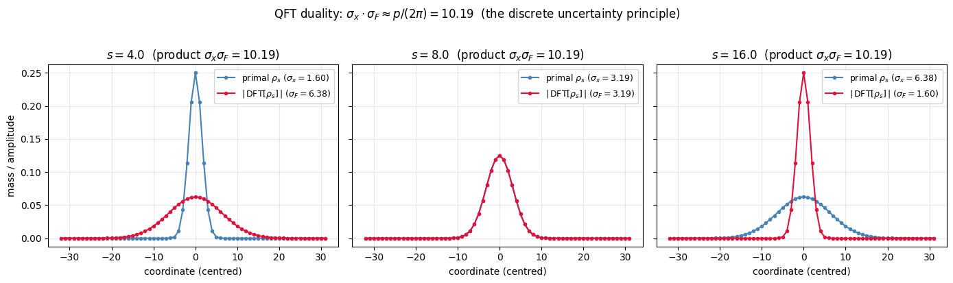
Connection to the main theorem
The product \(\sigma_x \cdot \sigma_{\hat x}\) stays approximately constant (the discrete-uncertainty principle). When Regev’s iteration gives us a “wide” Gaussian on \(L^*\) with parameter \(r\), applying the QFT yields a sample concentrated near \(L\) with parameter \(\sim 1/r\) — i.e. narrower. Iterating this trick is exactly how the proof ratchets down the noise.
50.6 The public-key cryptosystem (Section 4 of the paper)#
We can now read Section 4 of the paper line by line. Below is the spec verbatim from the paper, then a complete implementation.
Spec — Regev 2005, Section 4
Parameters. Choose \(m = 5n\) and \(p\) a prime in \([n^2, 2n^2]\). The noise distribution is \(\chi = \bar\Psi_{\alpha(n)}\) with \(\alpha(n) = o(1/\sqrt{n \log n})\) — concretely we take \(\alpha(n) = 1/(\sqrt n \log n)\).
Private key. Choose \(\mathbf{s} \in \mathbb{Z}_p^n\) uniformly at random.
Public key. For \(i = 1, \ldots, m\), choose \(\mathbf{a}_i \in \mathbb{Z}_p^n\) independently and uniformly, and \(e_i \sim \chi\) independently. The public key is
Encryption of a bit \(\mu \in \{0, 1\}\). Choose a random subset \(S \subseteq [m]\) (each index independently with probability 1/2). The ciphertext is
Decryption of \((\mathbf{a}, b)\). Compute \(d = b - \langle \mathbf{a}, \mathbf{s}\rangle \bmod p\) and lift to \((-p/2, p/2]\). Output 0 if \(|d| < p/4\), output 1 otherwise.
50.6.1 Why decryption works — the noise budget#
The honest ciphertext is
The accumulated error is the sum of \(|S|\) iid samples from \(\bar\Psi_\alpha\). Since each index is included in \(S\) independently with probability \(1/2\), we have \(\mathbb E[|S|] = m/2\), and using \(\mathrm{std}(\bar\Psi_\alpha) \approx \alpha p / \sqrt{2\pi}\) the total standard deviation is
Decryption fails only when this exceeds \(p/4\), i.e. when \(\alpha \gtrsim \sqrt{\pi}/(2\sqrt m)\). The asymptotic parameter choice \(\alpha = o(1/\sqrt{n\log n})\) keeps us safely below that threshold (recall \(m = 5n\)), so the failure probability is negligible.
50.6.2 Why it is IND-CPA secure#
Each of the \(m\) public-key rows is a fresh LWE sample. By the Decisional LWE assumption (which Regev establishes is equivalent to the search version), the public key is computationally indistinguishable from uniform. With a uniform public key, the ciphertext distribution for \(\mu = 0\) and \(\mu = 1\) differ only in the \(\lfloor p/2\rfloor\) offset added to the second component, which itself is statistically close to uniform whenever the sum of \(|S|\) uniform elements is. Composing, the cryptosystem is IND-CPA secure under LWE\(_{p, \bar\Psi_\alpha}\).
50.6.3 End-to-end implementation — Exercise#
def regev_keygen(n, p, m, alpha, rng):
    '''Generate Regev 2005 (sk, pk).  pk = (A, b),  A: m x n,  b: m.'''
    s = rng.integers(0, p, size=n)
    A = rng.integers(0, p, size=(m, n))
    e = psi_bar_alpha(alpha, p, rng, size=m)
    b = (A @ s + e) % p
    return s, (A, b)


def regev_encrypt(pk, mu, p, rng):
    '''Encrypt one bit mu in {0, 1}.  Ciphertext = (sum_S a_i, mu*floor(p/2) + sum_S b_i) mod p.'''
    A, b = pk
    m = A.shape[0]
    S = rng.integers(0, 2, size=m)          # uniform subset of [m]
    a_ct = (S @ A) % p
    b_ct = (int(S @ b) + int(mu) * (p // 2)) % p
    return a_ct, b_ct


def regev_decrypt(sk, ct, p):
    '''Decrypt (a, b).  Output 0 if |b - <a, s>|_centred < p/4, else 1.'''
    s = sk
    a, b = ct
    d = (int(b) - int(a @ s)) % p
    d_centred = d if d <= p // 2 else d - p
    return 0 if abs(d_centred) < p // 4 else 1


# Demo.  The paper's asymptotic alpha = 1/sqrt(n log n) is far too noisy
# for our tiny n=16 demo (sigma_total would exceed p/4 -> ~50% failures);
# we therefore use alpha = 1/(20 * sqrt(m)), which is comfortably below the
# decryption-failure threshold sigma_total = sqrt(m) * alpha * p / sqrt(2 pi)
# < p/4 derived in 50.6.1.  The security-vs-correctness trade-off is the
# focus of the next exercise (50.6.5).
def next_prime(x):
    def is_prime(k):
        if k < 2: return False
        for f in range(2, int(k ** 0.5) + 1):
            if k % f == 0: return False
        return True
    while not is_prime(x):
        x += 1
    return x

rng = np.random.default_rng(20260519)
n = 16
m = 5 * n                                                    # m = 5n
p = next_prime(n * n)                                        # smallest prime >= n^2
alpha = 1.0 / (20 * np.sqrt(m))                              # safely below failure threshold

sk, pk = regev_keygen(n, p, m, alpha, rng)
print(f'parameters n={n}, p={p}, m={m}, alpha={alpha:.4f}')
print(f'secret s    = {sk.tolist()}')

# Encrypt and decrypt 32 random bits, count failures.
n_trials = 200
failures = 0
for _ in range(n_trials):
    bit = int(rng.integers(0, 2))
    ct = regev_encrypt(pk, bit, p, rng)
    rec = regev_decrypt(sk, ct, p)
    if rec != bit:
        failures += 1
print(f'Decryption failures: {failures} / {n_trials}   (~{100 * failures / n_trials:.1f}%)')
parameters n=16, p=257, m=80, alpha=0.0056
secret s    = [241, 123, 127, 252, 43, 240, 203, 120, 89, 38, 52, 3, 33, 207, 109, 164]
Decryption failures: 0 / 200   (~0.0%)
50.6.4 Encrypt a multi-bit message — Exercise#
Encrypt the ASCII string “REGEV” bit by bit, store the ciphertexts, decrypt, and reconstruct the string.
message = "REGEV"
bits = [(ord(c) >> i) & 1 for c in message for i in range(7, -1, -1)]

cts = [regev_encrypt(pk, bit, p, rng) for bit in bits]
rec_bits = [regev_decrypt(sk, ct, p) for ct in cts]
rec_chars = [chr(sum(b << (7 - j) for j, b in enumerate(rec_bits[i:i+8])))
             for i in range(0, len(rec_bits), 8)]
recovered = ''.join(rec_chars)
print(f'plaintext   = {message!r}')
print(f'ciphertexts = {len(cts)}  (one per bit; each is a Z_p^{n+1} pair)')
print(f'recovered   = {recovered!r}   match = {recovered == message}')
print(f'ciphertext byte budget for one bit: '
      f'{(n + 1) * int(np.ceil(np.log2(p)))} bits  '
      f'(~{(n + 1) * int(np.ceil(np.log2(p))) / 8:.1f} bytes per plaintext bit)')
plaintext   = 'REGEV'
ciphertexts = 40  (one per bit; each is a Z_p^17 pair)
recovered   = 'REGEV'   match = True
ciphertext byte budget for one bit: 153 bits  (~19.1 bytes per plaintext bit)
50.6.5 Decryption failure rate as a function of \(\alpha\) — Exercise#
The total standard deviation derived in §50.6.1 is \(\sigma_{\text{total}} \approx \sqrt{m/2}\cdot \alpha p / \sqrt{2\pi}\). Setting this equal to the decision-boundary \(p/4\) gives the empirical failure-rate threshold
Below we sweep \(\alpha\) and measure the empirical failure rate; we expect a transition from \(\approx 0\) to \(\approx 50\%\) (random guessing) as \(\alpha\) crosses \(\alpha^*\).
rng = np.random.default_rng(2026)
n = 16
m = 5 * n
p = next_prime(n * n)

alphas = np.linspace(0.001, 0.08, 25)
trials_per_alpha = 300
rates = []
for a in alphas:
    sk_a, pk_a = regev_keygen(n, p, m, a, rng)
    fails = 0
    for _ in range(trials_per_alpha):
        bit = int(rng.integers(0, 2))
        ct = regev_encrypt(pk_a, bit, p, rng)
        if regev_decrypt(sk_a, ct, p) != bit: fails += 1
    rates.append(fails / trials_per_alpha)

# Theoretical breakdown: total stdev sqrt(m/2) * alpha * p / sqrt(2 pi)
# approaches the decision threshold p/4.  Solving for alpha gives the line
# below.  (We use m/2 because |S| ~ Binomial(m, 1/2) so E[|S|] = m/2.)
crit_alpha = (np.sqrt(2 * np.pi) / 4) / np.sqrt(m / 2)

fig, ax = plt.subplots(figsize=(8, 4.5))
ax.plot(alphas, rates, 'o-', color='steelblue', label='empirical decryption failure rate')
ax.axvline(crit_alpha, color='red', linestyle='--',
           label=fr'theory threshold  $\alpha^* \approx {crit_alpha:.3f}$')
ax.axhline(0.5, color='grey', linestyle=':', alpha=0.5, label='random guessing (50%)')
ax.set_xlabel(r'$\alpha$  (noise parameter)'); ax.set_ylabel('failure rate')
ax.set_title(fr'Regev cryptosystem: failure rate vs $\alpha$  ($n={n}$, $m={m}$, $p={p}$)')
ax.legend(); ax.grid(True, alpha=0.3)
plt.tight_layout(); plt.show()
print(f'threshold prediction: alpha* = sqrt(pi)/(2*sqrt(m)) = {crit_alpha:.4f}')

threshold prediction: alpha* = sqrt(pi)/(2*sqrt(m)) = 0.0991
50.7 Closing — from Regev 2005 to ML-KEM 2024#
The cryptosystem you just implemented is a bit-encryption scheme with a \(\tilde O(n^2)\)-bit public key and ciphertexts that blow up each plaintext bit by \(O(n \log n)\). The successor systems Kyber/ML-KEM (FIPS 203, 2024) make three structural improvements:
Improvement |
What it gains |
Where in the line |
|---|---|---|
Switch LWE → Ring-LWE over \(R_q = \mathbb{Z}_q[x]/(x^N+1)\) |
\(O(N \log q)\)-bit keys instead of \(O(N^2 \log q)\) |
Lyubashevsky–Peikert–Regev 2010 |
Module-LWE — interpolates between LWE and Ring-LWE |
tunable security / structure trade-off |
Langlois–Stehlé 2015 |
Encrypt \(N\) bits per ciphertext via polynomial ring |
constant amortised cost per bit |
Lyubashevsky–Peikert–Regev 2013 |
Use the Number Theoretic Transform for \(R_q\) multiplication |
\(O(N \log N)\) instead of \(O(N^2)\) |
Crystals-Kyber 2017 |
Fujisaki–Okamoto transform |
IND-CCA security from IND-CPA |
Bos et al. 2018 |
Every one of these changes preserves the worst-case to average-case reduction chain that Regev’s Theorem 1.1 established. That is why, two decades on, the post-quantum standard you will see your students implement in W3 is still recognisably the same algorithm you just coded.
Open questions
Can the quantum step in Theorem 1.1 be replaced by a classical reduction at the same parameters? Peikert (2009) and the Brakerski–Langlois–Peikert–Regev–Stehlé (2013) line of work classicalised the reduction in restricted parameter regimes; a matched classical version of Theorem 1.1 in full generality is still open as of 2024.
Can the hardness of LWE be reduced to the hardness of LPN (\(p = 2\))? Currently the best LPN-hardness assumption is much weaker than LWE’s, but every known reduction goes the other way.
For sub-exponential-time attacks on LWE, see Albrecht–Player–Scott (2015) and the Lattice Estimator. The cost models used by NIST for ML-KEM parameters are direct refinements of that estimator.
50.8 References#
Regev, O. (2005, 2009). On Lattices, Learning with Errors, Random Linear Codes, and Cryptography. STOC ‘05; J. ACM 56(6). The paper this tutorial follows. doi:10.1145/1060590.1060603 · in this repo as
sources/1060590.1060603.pdf.Blum, A., Kalai, A., Wasserman, H. (2003). Noise-tolerant learning, the parity problem, and the statistical query model. J. ACM 50(4), 506–519. The BKW algorithm.
Ajtai, M. (1996). Generating Hard Instances of Lattice Problems. STOC ‘96. The original worst-case to average-case reduction (for SIS, not LWE).
Lyubashevsky, V., Peikert, C., Regev, O. (2010). On Ideal Lattices and Learning with Errors over Rings. EUROCRYPT 2010. Ring-LWE.
Peikert, C. (2016). A Decade of Lattice Cryptography. Foundations and Trends in Theoretical Computer Science 10(4), 283–424. Survey, still the best single reference for the area.
Albrecht, M., Player, R., Scott, S. (2015). On the Concrete Hardness of Learning with Errors. J. Mathematical Cryptology 9(3). The “lattice estimator”.
NIST (2024). FIPS 203 — Module-Lattice-Based Key-Encapsulation Mechanism Standard. csrc.nist.gov/pubs/fips/203/final